| |
This is a series of typ;ical calculations made by tactical
commanders.
|
|
| |
(1) BASIC TIME AND DISTANCE CALCULATION
This simple formula is used for determining the approximate time required
to move a unit from one area to another, not counting the time required to move
out of the initial area and reach the start line. The information required is
the length of the march as measured from the initial starting line (SL) (at a
distance outside the original assembly area) to the nearest point of the new
assembly area; the average rate of march of the column, the length of time
spent in halts, and the time required to deploy from the road into the new
area.
The formula is:
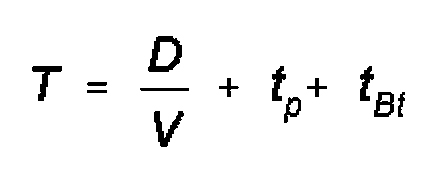
where:
tBt=is computed if the depth of new area is less than depth of the
march formation.
t=total time of march;
D=length of route;
V=average speed of column on march in kph;
tp=overall time for halts during march;
tBt=time required to deploy into new area;
|
|
| |
(2) CALCULATION OF TIME TO BEGIN MOVE TO
START LINE
This calculation is used to determine when a unit should begin moving out
of its assembly area in order for the head of the column to cross the start
line (SL) at the prescribed time. The given data are the distance from the
assembly area to the start line and the rate of march. The formula is:
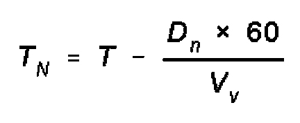
where:
Dn=distance to SL;
tN=time column starts to move;
Vv=rate of movement to SL;
60=conversion factor Hr to min;
T=time head of column passes SL;
|
|
| |
(3) CALCULATION OF TIME TO DEPLOY INTO NEW
ASSEMBLY AREA
As noted in formula (1), this only must be calculated when the depth of the
new area is less than the length of the mobile column. This is because in this
case the head of the column will have stopped at the far end before the tail
reaches the near side of the area. The formula gives the time it takes to
deploy, once the head of the column has reached the new area.The formula is:
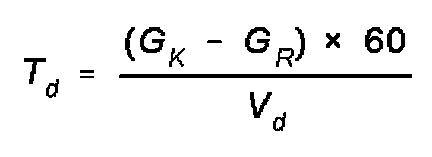
where:
Td=time for deployment;
GK=length of column;
GR=depth of area;
Vd=speed during deployment;
60=convert hr to min;
|
|
| |
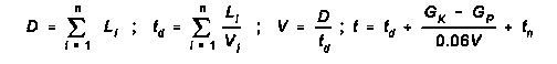
(4) CALCULATION OF TIME A UNIT WILL BE IN A
NEW AREA
This calculation combines the previous formulas in order to determine the
clock time a unit will be deployed in the new area. It takes into consideration
the time required for a unit to deploy into an area when the depth of that area
is less than the length of the marching column. It also includes time for halts
en route. Formula of calculation:
 where:
t=clock time a unit will be regrouped in new area in hrs;
T=time (astronomical) of passing start point (line) by front of column in
hrs/mins;
D=length of route and distance away of new concentration area in km;
V=average speed of movement;
GK=length of column;
GR=depth of new concentration area in km (considered only when the
depth is less than the length of column);
0.6=coefficient, which takes into account the lowering of the average march
speed while deploying into the new assembly area.
tp=duration of halts en route in hrs.
This calculation may be conveniently performed by entering the data into a
table.
|
|
| |
CALCULATION OF TIME UNIT IS ASSEMBLED IN NEW AREA
|
| No |
Initial data and values to be calculated |
Units |
Calculation variant |
Remarks |
| Example |
2 |
3 |
4 |
| 1 |
Length of march route |
km |
167 |
|
|
|
|
| 2 |
Average rate of movement |
|
18 |
|
|
|
|
| 3 |
Length of moving column |
|
7.5 |
|
|
|
|
| 4 |
Depth of new assembly area |
|
4 |
|
|
|
|
| 5 |
Duration of halts |
|
1.5 |
|
|
|
|
| 6 |
Time of passing start line (SL) |
|
10.0 |
|
|
|
|
| 7 |
(1) ÷ (2) |
|
9.3 |
|
|
|
|
| 8 |
(3) - (4) |
0.1 |
3.5 |
|
|
|
|
| 9 |
(2) x 0.6 |
0.1 |
10.8 |
|
|
|
|
| 10 |
(8) ÷ (9) |
0.1 |
0.3 |
|
|
|
|
| 11 |
Overall duration of march (5) + (7) + (10)
|
0.1 |
11.1 |
|
|
|
|
| 12 |
Time unit is concentrated in new area (6) + (11) |
hrs |
21:06 |
|
|
|
|
|
|
| |
|
CALCULATION OF TIME UNIT IS ASSEMBLED IN NEW AREA
|
| No |
Initial data and values to be calculated |
Units |
Calculation variant
|
Remarks |
| 1 |
2 |
3 |
4 |
| 1 |
Length of march route |
km |
|
|
|
|
|
| 2 |
Average rate of movement |
|
|
|
|
|
|
| 3 |
Length of moving column |
|
|
|
|
|
|
| 4 |
Depth of new assembly area |
|
|
|
|
|
|
| 5 |
Duration of halts |
|
|
|
|
|
|
| 6 |
Time of passing start line (SL) |
|
|
|
|
|
|
| 7 |
(1) ÷ (2) |
|
|
|
|
|
|
| 8 |
(3) - (4) |
0.1 |
|
|
|
|
|
| 9 |
(2) x 0.6 |
0.1 |
|
|
|
|
|
| 10 |
(8) ÷ (9) |
0.1 |
|
|
|
|
|
| 11 |
Overall duration of march (5) + (7) + (10)
|
0.1 |
|
|
|
|
|
| 12 |
Time unit is concentrated in new area (6) + (11) |
hrs |
|
|
|
|
|
|
|
| |
(5) CALCULATION OF MARCH DURATION FROM ONE AREA TO ANOTHER
This is a more sophisticated version of the basic march formula to take account
of possible reductions in the capacity of the road or other influences on the
achievable rate of movement of the columns. The formula is:
 when GK > Gr
where:
t=duration of march in hours;
D=length of march in km;
K=coefficient for reduction in average rate of march of moving columns during
entering and leaving the route of march;
Di=distance of start point from original assembly area in km;
GK=depth of column in km;
Gr=depth of the new assembly area in km;
V=average rate of movement of column in km/hr;
tp=duration of halts or delays during movement in hrs.
|
|
| |
TABLE FOR CALCULATING DURATION OF A MARCH
|
| No |
Initial data and values to be determined |
Units |
Calculation variant |
Remarks |
| Example |
2 |
3 |
| 1 |
Route length |
km |
87 |
|
|
|
| 2 |
Speed reduction factor |
-- |
0.6 |
|
|
(1) x (2) |
| 3 |
Distance to start point |
km |
4.5 |
|
|
+ (3) |
| 4 |
Column depth |
km |
11.2 |
|
|
+ (4) |
| 5 |
Depth of new concentration region |
km |
7 |
|
|
- (5) |
| 6 |
Rate of march |
km/hr |
18 |
|
|
÷ (6) |
| 7 |
Speed reduction factor |
-- |
0.6 |
|
|
÷ (7) |
| 8 |
Length of halts |
hr |
1 |
|
|
+ (8) |
| 9 |
March duration |
hr |
6.64 |
|
|
=ans |
|
|
| |
TABLE FOR CALCULATING DURATION OF A MARCH
|
| No |
Initial data and values to be determined |
Units |
Calculation variant
|
Remarks |
| 1 |
2 |
3 |
| 1 |
Route length |
km |
|
|
|
|
| 2 |
Speed reduction factor |
-- |
|
|
|
(1) x (2) |
| 3 |
Distance to start point |
km |
|
|
|
+ (3) |
| 4 |
Column depth |
km |
|
|
|
+ (4) |
| 5 |
Depth of new concentration region |
km |
|
|
|
- (5) |
| 6 |
Rate of march |
km/hr |
|
|
|
÷ (6) |
| 7 |
Speed reduction factor |
-- |
|
|
|
÷ (7) |
| 8 |
Length of halts |
hr |
|
|
|
+ (8) |
| 9 |
March duration |
hr |
|
|
|
=ans |
|
|
| |
(6) DETERMINE THE REQUIRED MOVEMENT RATE FOR A UNIT TO
REGROUP IN A NEW AREA
This is a more elaborate version of the basic movement formulas to take
into account more variables and possible interactions during the movement. The
formula is:

|
|
| |
|
FORM FOR CALCULATING REQUIRED TRAVEL SPEED
|
| No |
Initial data and values to be determined |
Units |
Calculation variant |
Remarks |
| Example |
2 |
3 |
| 1 |
Route length |
km |
128 |
|
|
|
| 2 |
Speed reduction factor |
-- |
0.7 |
|
|
|
| 3 |
Distance to start point |
km |
4.5 |
|
|
|
| 4 |
Column depth |
km |
8.7 |
|
|
|
| 5 |
Depth of concentration area |
km |
5.5 |
|
|
|
| 6 |
Maximum travel time allowed |
hr |
6 |
|
|
|
| 7 |
Halt time |
hr |
0.75 |
|
|
|
| 8 |
Speed reduction factor |
-- |
0.7 |
|
|
|
| 9 |
Required travel speed |
km/hr |
27 |
|
|
|
|
|
| |
FORM FOR CALCULATING REQUIRED TRAVEL SPEED
|
| No |
Initial data and values to be determined |
Units |
Calculation variant
|
Remarks |
| 1 |
2 |
3 |
| 1 |
Route length |
km |
|
|
|
|
| 2 |
Speed reduction factor |
-- |
|
|
|
|
| 3 |
Distance to start point |
km |
|
|
|
|
| 4 |
Column depth |
km |
|
|
|
|
| 5 |
Depth of concentration area |
km |
|
|
|
|
| 6 |
Maximum travel time allowed |
hr |
|
|
|
|
| 7 |
Halt time |
hr |
|
|
|
|
| 8 |
Speed reduction factor |
-- |
|
|
|
|
| 9 |
Required travel speed |
km/hr |
|
|
|
|
|
|
| |
(7) CALCULATION OF LENGTH OF ROUTE, AVERAGE SPEED AND
DURATION OF MOVEMENT OF MOVING COLUMN
This calculation combines the basic equations. It is used when the total
distance to be traveled is composed of segments having different route
characteristics. The different characteristics result in different possible
movement rates over the individual sectors. The initial data is the length of
each sector, the movement rate over each sector, the length of the column and
the depth of the new assembly area. Formulas for calculation:

where:
D=length of route in km;
Li=length of each sector of different types of road each allowing
Vi speed of movement of columns in km;
td=overall time on the route in hrs;
Vi=speed of movement on a type of sector of the route in kph;
V=average speed of movement in kph.
GK=length of column in km;
GP=depth of concentration area in km;
0.6=coefficient of reduction in speed of the column while deploying into the
new area or depending on local conditions;
tn=overall time of halts.
|
|
| |
|
CALCULATION OF TRANSIT TIME OVER MULTI-SEGMENT ROUTE
|
| No |
Initial data - form of calculations |
Units |
Calculation variants |
Remarks |
| Example |
2 |
3 |
| 1 |
Length of paved roads |
km |
42 |
|
|
|
| 2 |
Speed of movement on 1 |
km/hr |
35 |
|
|
|
| 3 |
Length of improved dirt roads |
km |
18 |
|
|
|
| 4 |
Speed of movement on 3 |
km/hr |
25 |
|
|
|
| 5 |
Length of dirt roads |
km |
21 |
|
|
|
| 6 |
Speed of movement on 5 |
km/hr |
15 |
|
|
|
| 7 |
Length of field tracks |
km |
8 |
|
|
|
| 8 |
Speed of movement on 7 |
km/hr |
10 |
|
|
|
| 9 |
Length of moving column |
km |
6.8 |
|
|
|
| 10 |
Depth of new assembly area |
km |
3 |
|
|
|
| 11 |
Overall time for halts |
hr |
1.5 |
|
|
|
| 12 |
Total length of route (1) + (2) + (5) + (7)
|
km |
89 |
|
|
|
| 13 |
(1) ÷ (2) |
|
1.2 |
|
|
|
| 14 |
(3) ÷ ((4) |
|
.7 |
|
|
|
| 15 |
(5) ÷ (6) |
|
1.4 |
|
|
|
| 16 |
(7) ÷ (8) |
|
0.8 |
|
|
|
| 17 |
Time of movement (13) + (14) + (15) + (16)
|
hr |
4.1 |
|
|
|
| 18 |
Average speed (12) ÷ (17) |
km/hr |
22 |
|
|
|
| 19 |
(9) - (10) ÷ [0.6 x (18)] |
|
3.8 |
|
|
|
| 20 |
Time of deploy - new area (19) ÷ [0.6 x (18)]
|
hr |
.3 |
|
|
|
| 21 |
Duration of move (11) + (17) + (20)
|
|
5.9 |
|
|
|
|
|
| |
|
CALCULATION OF TRANSIT TIME OVER MULTI-SEGMENT ROUTE
|
| No |
Initial data - form of calculations |
Units |
Calculation variants |
Remarks |
| 1 |
2 |
3 |
| 1 |
Length of paved roads |
km |
|
|
|
|
| 2 |
Speed of movement on 1 |
km/hr |
|
|
|
|
| 3 |
Length of improved dirt roads |
km |
|
|
|
|
| 4 |
Speed of movement on 3 |
km/hr |
|
|
|
|
| 5 |
Length of dirt roads |
km |
|
|
|
|
| 6 |
Speed of movement on 5 |
km/hr |
|
|
|
|
| 7 |
Length of field tracks |
km |
|
|
|
|
| 8 |
Speed of movement on 7 |
km/hr |
|
|
|
|
| 9 |
Length of moving column |
km |
|
|
|
|
| 10 |
Depth of new assembly area |
km |
|
|
|
|
| 11 |
Overall time for halts |
hr |
|
|
|
|
| 12 |
Total length of route (1) + (2) + (5) + (7)
|
km |
|
|
|
|
| 13 |
(1) ÷ (2) |
|
|
|
|
|
| 14 |
(3) ÷ ((4) |
|
|
|
|
|
| 15 |
(5) ÷ (6) |
|
|
|
|
|
| 16 |
(7) ÷ (8) |
|
|
|
|
|
| 17 |
Time of movement (13) + (14) + (15) + (16)
|
hr |
|
|
|
|
| 18 |
Average speed (12) ÷ (17) |
km/hr |
|
|
|
|
| 19 |
(9) - (10) ÷ [0.6 x (18)] |
|
|
|
|
|
| 20 |
Time of deploy - new area (19) ÷ [0.6 x (18)]
|
hr |
|
|
|
|
| 21 |
Duration of move (11) + (17) + (20)
|
|
|
|
|
|
|
|
| |
(8) CALCULATION OF OVERALL DEPTH OF COLUMN
CONSISTING OF SEVERAL SUB-COLUMNS
This technique is for calculating the total length of a moving formation on
a route given the number of vehicles in the moving columns and the distances
between them is known. It is also used to determine the required distances
between vehicles. The formula is:
 where:
Gk=formation depth in km;
Nm=number of vehicles;
dm=distance between vehicles;
NK=number of columns;
dK=distance between columns;
1000=convert meter to km.
|
|
| |
(9) CALCULATION OF DURATION OF PASSAGE OF
NARROW POINTS AND DIFFICULT SEGMENTS
This calculation is the basic one for determining the time it will take a
column of given length to pass through a constriction in the route. It does not
take into consideration the issue of vehicle bunching up at the halt before the
constriction nor the time to regain column vehicle separation distances after
the passage. Therefore more elaborate formulas are used to determine the
overall effect of a constriction on a full march. The formula for short
obstacles is:
 where:
Nm=number of vehicles;
dm=distance between vehicles;
t=time required to overcome obstacle in minutes;
V=speed of column through obstacle;
0.06=conversion factor km/hr to meters/min.
The formula for major obstacles:
 where:
Gk=length of column;
D=length negotiated segment;
t=duration to overcome obstacle in hours;
v=speed through obstacle.
|
|
| |
(10) CALCULATION FOR PASSAGE TIMES ACROSS
START POINT (SL) BY THE HEAD AND TAIL OF THE COLUMN
This calculation also determines the time for a column to pass a given
point, however, since there is no delay as with an obstacle, the time interval
is governed by the length of the column and its velocity. Since we are not
interested in the length of time the column requires, but the clock times the
head and tail cross, the equations yield time in military time. The formula is:
 where:
ti=SL crossing time of the head of the march column i in hours and minutes;
Ti-1=the time for passing the line by the tail of the leading march
column in hours and minutes; for the head of the first column this time is the
time specified for passing the line by the head of the entire formation, for
instance, by the column of the leading unit on a route;
di=the specified distance between the lead and the i march column in
km;
60=factor for converting hours into minutes;
V=average speed in km per hr;
t'i=the time for passing the line by the tail of the i route column
in hours and minutes;
Di=depth of the i column in km.
|
|
| |
(11) CALCULATION OF EXPECTED TIME AND
DISTANCE OF PROBABLE POINT OF CONTACT WITH ADVANCING ENEMY
Clearly this is one of the most important calculations Soviet commander's
make regularly during the course of combat. As the discussion of meeting
engagements in Chapters One and Two indicates, the commander's effort to
control the flow of battle focuses heavily on the relative times and place of
introduction of his second echelon versus the enemy's reserves, both of which
are moving forward.
The formula is:
 where:
te=expected tome of meeting in hours;
D=initial distance between opposing groupings in km;
Vf=movement rate of friendly troops in km per hr;
Ve=movement rate of enemy forces in km per hr;
dl=distance from friendly initial position to expected point of
contact in km;
|
|
| |
(12) CALCULATION OF TIME REQUIRED FOR
ADVANCING AND DEPLOYING SUB-UNITS TO CHANGE FROM LINE OF MARCH INTO THE ATTACK
Determination of the time a unit should begin to move for the advance from
its assembly area to the line of commitment into battle and assault on the
enemy position is a complex application of the basic time and distance formula.
All times are measured backwards from "CHE" hour, the moment the
troops hit the first line of the defending enemy's position. The total time
from beginning of movement in the assembly area is composed of the segments of
time while moving in each type of deployment, that is: line of attack, company
column, battalion column, and regimental column. It also includes the time it
takes to shift from one formation to the other and any time for halts and
delays en route. This is one of the most important and fundamental of tactical
calculations. The times for sub-unit movement are tied exactly into the times
for the artillery preparatory fire and air strikes.
The required given data are the distances between each of the deployment
and regulating lines, distance of the attack line from the enemy's forward line
of defense, distance of the start line from the unit assembly area, the average
speed of movement while mounted in the columns, the coefficient for speed
reduction during deployment actions, the speed of movement in attack formation,
the depth of the columns, and distance between first and second echelons of the
units.
|
|
| |
(12) CALCULATION OF TIME REQUIRED FOR
ADVANCING AND DEPLOYING SUB-UNITS TO CHANGE FROM LINE OF MARCH INTO THE ATTACK
The set of formulas are:


 where:
ta=time for crossing final deployment into line of attack -
"Che" hour -in minutes;
Da=distance of line for going into attack formation from the forward
edge of the enemy position in km;
Va=rate of movement in attack formation in kph;
tr=time for crossing the line of deployment into company columns at
("Che" - minutes)
Dr=distance of line of deployment into company columns from the line
of deployment into attack formation in km;
V=average rate of movement of subunits in mounted formation during march;
tb=time for crossing line of deployment into battalion columns at
("Che" - minutes);
Db=distance of line for deployment into battalion columns from line
of deployment into company columns in km;
trr=time for crossing the last regulation line or point prior to the
deployment into battalion columns;
Drr=distance of last regulation line from the line for deployment
into battalion columns;
ti=time for passing the start line at ("Che" - minutes)
Di=distance of start line from last regulating line in km;
tvit=time to begin movement of subunits in assembly area;
D=distance of start line from the last unit assembly area;
t'i=time for crossing the start line by the 2nd echelon
of units at ("Che" - minutes);
Gk=depth of the mounted column of first echelon of units in km;
dk=distance between the tail of the first echelon and head of the
2nd echelon of the units in km;
The numbers 60 and 90 are coefficients for conversion of time in minutes for
the average speed of movement during the deployment of the units at each of the
lines. For example, the 90 shows that the average maneuver speed of the unit
during the actual deployment on a line decreases by a factor of 1.5 in
comparison with the speed of forward movement between the lines. Depending on
the concrete conditions and situation for movement on the terrain, this could
be some other factor.
To perform the calculation the required data may be entered into the table. The
result will be the planning data for start of forward movement and deployment
times for each shift of sub-unit columns. Since all times are measured backward
from "Che", the planner must remember to subtract the values
indicated in lines 12, 15, 18, 21, 24, and 27 from Che; and add the value for
time in line 30 to the time in 24 to obtain line 31.
|
|
| |
CALCULATION OF TIME TO ADVANCE AND DEPLOY SUB-UNITS FOR SHIFT INTO ATTACK
FROM LINE OF MARCH
|
| No |
Initial data, values and calculations to
perform |
Units Precision |
Calculation variant |
| 1 |
2 |
3 |
| 1 |
2 |
3 |
4 |
5 |
6 |
| 1 |
Distance of attack line from enemy front line |
|
|
|
|
| 2 |
Distance of line to deploy into company columns from attack
line |
|
|
|
|
| 3 |
Distance of line to deploy into battalion columns from line of
company columns |
|
|
|
|
| 4 |
Distance of regulation line from line to deploy into battalion
columns |
|
|
|
|
| 5 |
Distance of regulation line from start line |
|
|
|
|
| 6 |
Distance of start line from the unit assembly (FUP) area |
|
|
|
|
| 7 |
Movement speed into the attack |
|
|
|
|
| 8 |
Average speed during march |
|
|
|
|
| 9 |
Dept of first echelon march column |
|
|
|
|
| 10 |
Interval between first and second echelon columns |
|
|
|
|
| 11 |
(1) x 60 |
|
|
|
|
| 12 |
Time to cross line for shifting to attack (Che - min) (11)
÷ (7)
|
|
|
|
|
| 13 |
(2) x 90 |
|
|
|
|
| 14 |
(13) ÷ (8) |
|
|
|
|
| 15 |
Time to cross line of deployment into company columns: (Ch - )
(12) + (14) |
|
|
|
|
| 16 |
(3) x 60 |
|
|
|
|
| 17 |
(16) ÷ (8) |
|
|
|
|
| 18 |
Time to cross line of deployment into battalion columns: (Ch -
) (15) + (17) |
|
|
|
|
| 19 |
(4) x 60 |
|
|
|
|
| 20 |
(19) ÷ (8) |
|
|
|
|
| 21 |
Time to cross regulation line (Ch - ) (18) + 20)
|
|
|
|
|
| 22 |
(5) x 60 |
|
|
|
|
| 23 |
(22) ÷ (8) |
|
|
|
|
| 24 |
Time to cross start line (Ch - ) (21) + (23) |
|
|
|
|
| 25 |
(6) x 90 |
|
|
|
|
| 26 |
(25) ÷ (8) |
|
|
|
|
| 27 |
Time to start moving out of assembly area - 1st echelon (Ch - )
(24) + (26) |
|
|
|
|
| 28 |
(9) + (10) |
|
|
|
|
| 29 |
(28) x 90 |
|
|
|
|
| 30 |
(29) ÷ (8) |
|
|
|
|
| 31 |
Time for second echelon to pass start line (SL) (Ch - ) (24) -
(30) |
|
|
|
|
|
|
| |
CALCULATION OF TIME TO ADVANCE AND DEPLOY SUB-UNITS FOR SHIFT INTO ATTACK
FROM LINE OF MARCH
|
| No |
Initial data, values and calculations to
perform |
Units Precision |
Calculation variant |
| 1 |
2 |
3 |
| 1 |
2 |
3 |
4 |
5 |
6 |
| 1 |
Distance of attack line from enemy front line |
|
|
|
|
| 2 |
Distance of line to deploy into company columns from attack line |
|
|
|
|
| 3 |
Distance of line to deploy into battalion columns from line of company
columns |
|
|
|
|
| 4 |
Distance of regulation line from line to deploy into battalion columns |
|
|
|
|
| 5 |
Distance of regulation line from start line |
|
|
|
|
| 6 |
Distance of start line from the unit assembly (FUP) area |
|
|
|
|
| 7 |
Movement speed into the attack |
|
|
|
|
| 8 |
Average speed during march |
|
|
|
|
| 9 |
Dept of first echelon march column |
|
|
|
|
| 10 |
Interval between first and second echelon columns |
|
|
|
|
| 11 |
(1) x 60 |
|
|
|
|
| 12 |
Time to cross line for shifting to attack (Che - min) (11) ÷ (7)
|
|
|
|
|
| 13 |
(2) x 90 |
|
|
|
|
| 14 |
(13) ÷ (8) |
|
|
|
|
| 15 |
Time to cross line of deployment into company columns: (Ch - ) (12) + (14)
|
|
|
|
|
| 16 |
(3) x 60 |
|
|
|
|
| 17 |
(16) ÷ (8) |
|
|
|
|
| 18 |
Time to cross line of deployment into battalion columns: (Ch - ) (15) +
(17) |
|
|
|
|
| 19 |
(4) x 60 |
|
|
|
|
| 20 |
(19) ÷ (8) |
|
|
|
|
| 21 |
Time to cross regulation line (Ch - ) (18) + 20)
|
|
|
|
|
| 22 |
(5) x 60 |
|
|
|
|
| 23 |
(22) ÷ (8) |
|
|
|
|
| 24 |
Time to cross start line (Ch - ) (21) + (23) |
|
|
|
|
| 25 |
(6) x 90 |
|
|
|
|
| 26 |
(25) ÷ (8) |
|
|
|
|
| 27 |
Time to start moving out of assembly area - 1st echelon (Ch - ) (24) +
(26) |
|
|
|
|
| 28 |
(9) + (10) |
|
|
|
|
| 29 |
(28) x 90 |
|
|
|
|
| 30 |
(29) ÷ (8) |
|
|
|
|
| 31 |
Time for second echelon to pass start line (SL) (Ch - ) (24) - (30) |
|
|
|
|
|
|
| |
(13) CALCULATION OF THE TIME AND DISTANCE
TO THE LINE OF CONTACT
This method takes into consideration the many situational factors that are
ignored in the simpler formula and nomogram. In fact, there are so many
possible influences on the time the two sides will meet and hence the location
of meeting that a nomogram can only give a crude approximation of the answer.
With the use of computers or even hand calculators and an established procedure
such as that shown in this table it is possible to assess the influence of many
more factors.
The set of formulas is:
tv={D + [(tn x Vn) +
(tp x Vp)]} ÷ (Vn +
Vp)
Tn=t1 + t2 t3;
TP=t1' + t2' + t3'
where:
tv=expected time if contact with enemy in hours;
D=distance between forces of the two sides in km;
tn=total delay time for own force in hrs;
Vn=speed movement of own forces in km per hr;
tp=total delay time of enemy in hrs;
Vp=speed movement of enemy in km per hr;
lp=distance to expected line of meeting with enemy;
t1 (t'1)=delay - (time difference) start of
movement of one side versus other in hrs;
t2 (t'2=duration of halts of forces of each
side in hrs;
t3 (t'3)=duration of delay of forces due to
strikes by opponent en route in hrs;
|
|
| |
CALCULATION OF EXPECTED TIME AND DISTANCE TO PROBABLE LINE OF MEETING
ENGAGEMENT
|
| No |
Initial data, values and calculations |
Units Precision |
Calculation variant |
| Example |
2 |
3 |
| 1 |
2 |
3 |
4 |
5 |
6 |
| 1 |
Friendly force starts advance |
hr, min |
20:00 |
|
|
| 2 |
Enemy force starts advance |
hr, min |
21:00 |
|
|
| 3 |
Distance between opponents at start |
km (1.0) |
105 |
|
|
| 4 |
Delay in advance of friendly relative to enemy |
hr (0.1) if 1 > 2
|
-- |
|
|
| 5 |
Total duration of halts of friendly |
hr (0.1) |
0.3 |
|
|
| 6 |
Total duration of delays of friendly by enemy |
hr (0.1) |
-- |
|
|
| 7 |
Friendly force travel speed |
km/hr (1.0) |
28 |
|
|
| 8 |
Delay of enemy start relative to friendly |
hr (0.1) if 2 > 1
|
1 |
|
|
| 9 |
Total duration of halts of enemy |
hr (0.1) |
0.5 |
|
|
| 10 |
Total duration of delays of enemy due to friendly |
hr (0.1) |
0.6 |
|
|
| 11 |
Enemy force travel speed |
km/hr (1.0) |
19 |
|
|
| 12 |
(4) + (5) + (6) |
(0.1) |
0.3 |
|
|
| 13 |
(12) x (7) |
(0.1) |
8.4 |
|
|
| 14 |
(8) + (9) + (10) |
(1.0) |
2.1 |
|
|
| 15 |
(14) x (11) |
(1.0) |
40 |
|
|
| 16 |
(3) + (13) + (15) |
(1.0) |
153 |
|
|
| 17 |
(7) + (11) |
(0.1) |
47 |
|
|
| 18 |
Expected time of meeting (relative) (16) ÷ (17)
|
hr (0.1) |
3.3 |
|
|
| 19 |
Duration of travel time to meeting line: (18) - (12) |
hr (0.1) |
3 |
|
|
| 20 |
Distance to meeting line: (19) x (7)
|
km (1.0) |
84 |
|
|
|
|
| |
CALCULATION OF EXPECTED TIME AND DISTANCE TO PROBABLE LINE OF MEETING
ENGAGEMENT
|
| No |
Initial data, values and calculations |
Units Precision |
Calculation variant |
| Example |
2 |
3 |
| 1 |
2 |
3 |
4 |
5 |
6 |
| 1 |
Friendly force starts advance |
hr, min |
|
|
|
| 2 |
Enemy force starts advance |
hr, min |
|
|
|
| 3 |
Distance between opponents at start |
km (1.0) |
|
|
|
| 4 |
Delay in advance of friendly relative to enemy |
hr (0.1) if 1 > 2
|
- |
|
|
| 5 |
Total duration of halts of friendly |
hr (0.1) |
|
|
|
| 6 |
Total duration of delays of friendly by enemy |
hr (0.1) |
- |
|
|
| 7 |
Friendly force travel speed |
km/hr (1.0) |
|
|
|
| 8 |
Delay of enemy start relative to friendly |
hr (0.1) if 2 > 1
|
|
|
|
| 9 |
Total duration of halts of enemy |
hr (0.1) |
|
|
|
| 10 |
Total duration of delays of enemy due to friendly |
hr (0.1) |
|
|
|
| 11 |
Enemy force travel speed |
km/hr (1.0) |
|
|
|
| 12 |
(4) + (5) + (6) |
(0.1) |
|
|
|
| 13 |
(12) x (7) |
(0.1) |
|
|
|
| 14 |
(8) + (9) + (10) |
(1.0) |
|
|
|
| 15 |
(14) x (11) |
(1.0) |
|
|
|
| 16 |
(3) + (13) + (15) |
(1.0) |
|
|
|
| 17 |
(7) + (11) |
(0.1) |
|
|
|
| 18 |
Expected time of meeting (relative) (16) ÷ (17)
|
hr (0.1) |
|
|
|
| 19 |
Duration of travel time to meeting line: (18) - (12) |
hr (0.1) |
|
|
|
| 20 |
Distance to meeting line: (19) x (7)
|
km (1.0) |
|
|
|
|
|
| |
(14) CALCULATION OF EXPECTED TIME AND RATE
OF OVERTAKING WHEN PURSUING THE ENEMY
Naturally the commander hopes to use this calculation often! The initial
data are the distance between the enemy and friendly forces, the average travel
speed of friendly and enemy forces, or the ordered time to overtake him. The
formula is:
 where:
to=time to overtake enemy in hours;
D=distance to the enemy in km;
Vn=friendly speed in pursuit in km per hr;
Vp=enemy speed in retreat in km per hr;
|
|
| |
(15) CALCULATION OF THE WORK TIME AVAILABLE
TO THE COMMANDER AND STAFF FOR ORGANIZING REPULSE OF ADVANCING ENEMY FORCES
This is obviously a critical issue in meeting engagements and encounter
battle. It is also relevant to defensive situations when preparing fire on the
attacker. The method is designed to determine the time the commander and staff
will have to organize the enemy's defeat by firing on the advancing forces
relative to the distance to the enemy, the speed of his advance, the effective
range of friendly weapons and the time required to prepare the sub-units to
fire. In this example it is assumed that the enemy will be taken under fire
beginning at the maximum range of the firing weapons. The formula is:
 where:
t=time available for commander and his staff to organize repelling the
advancing force in minutes;
D=distance to advancing enemy km;
d=max range of friendly weapons km;
60=conversion factor hours to minutes;
Ve=rate of enemy advance kph;
tp=time required to prepare subunits to destroy enemy with fire in
minutes;
|
|
| |
(17) DETERMINATION OF QUANTITY OF VARIOUS
WEAPONS, RECONNAISSANCE, SUPPORT, COMMUNICATIONS ETC. FOR TASK PERFORMANCE
This general technique is applicable to a wide variety of activities in
which it is desired to know what the overall effectiveness of a group of agents
will be when the probability of success of an individual agent is known. First
one calculates the action of the number of identical equipments, and then
determines the total effectiveness or total requirement for the systems. the
initial data for the calculations are information about the number of available
systems, the assigned degree of success for each, the effectiveness of the
systems (which is expressed in probability of mission fulfillment or by the
mean value of the applied damage to a particular target.) A single system also
means a complex of systems combined into a whole unit. Such data, for instance,
are the probability of target destruction, the man damage applied to an enemy
target, the reliability of a communications channel, the probability of enemy
target detection, the probability of the flawless operation of a water crossing
for a specific time interval, the probability of overcoming the anti-air forces
of the enemy and so on. These data may be obtained on the basis of the results
of studies, from statistical data nd from tactical and technical
characteristics.
The formulas for calculating the degree of mission fulfillment by a designated
number of systems is expressed through mission fulfillment probability:
 and through the mathematical expectation (mean
value) of damage:

 where:
Pn=probability of mission accomplished by a homogenous group of
weapons;
P1=same by a single system;
Mn=average (mean) value of damage inflicted on the enemy by a group
of systems;
M1=average value of damage inflicted on the enemy by one system;
n=quantity of available systems.
The formulas for computing the required number of systems when the
effectiveness of the systems is expressed by probability of task performance
is:

when Pn > P1
 when it is expressed by the mathematical
expectation (the mean value) of the inflicted damage, the formula is:

 when Mn > M1
The formula for calculating the effectiveness of different systems
fulfilling a common mission is :

where Pn is the overall effectiveness of systems used or in other
words the likelihood of fulfilling the mission, and the individual
"P"'s are the effectiveness measures of each system being summed for
the task.
From these examples it is evident that the technique may be used for
calculating a wide range of direct and inverse problems associated with the use
of various forces and means. With proper additional factors this method may
also be used to calculate rapidly the effectiveness and required number of
forces and systems when taking into account also probable enemy
countermeasures.
The formulas for calculating the effectiveness of forces and means with
consideration for probable enemy countermeasures are:

 where:
Pn=the probability of mission fulfillment by a group of systems;
P1=the probability of mission fulfillment by a single system of this
type;
Q=the probability indicator of the enemy countermeasure ;
n=the number of forces and means of the given type;
Mn=the mathematical expectation of the damage inflicted by a single
system of this type'
|
|
| |
(18) Modeling battle
There is much discussion in the Soviet literature about the theory of
development of coefficients of comensurability. The coefficient is designed to
make it possible to aggregate the effective contribution of various weapons to
a combined arms battle into a composite score for each side. This makes the
measurement of the correlation of forces relatively simple, ie. only one number
for each side rather than the long list of individual types of weapons found in
the standard tables of correlation of forces. However, what sounds simple in
theory is quite difficult in practice. Soviet authors point out that even
within types of weapons such as tanks or artillery the "proving ground
scores" assigned on the basis of technical/tactical characteristics may
not be true reflections of the actual value of the weapon to the commander in
all the diverse conditions of real combat. When it comes to establishing a
uniform score that will place tanks, artillery, aircraft, and small arms, etc
on one scale; a lot of judgment is involved. There is some argument for two
different methods, one would develop a "average" score for each
weapon reflecting its varied value in different circumstances, and the other
method would establish a single theoretical value number and then provide
situation modifiers to be applied to account for each actual set of combat
conditions. We do not have available an actual set of Soviet "utils"
as they call their weapons scores. The following table is taken from a Soviet
article, but the scores are purely hypothetical for educational purposes.
Nevertheless, the following method represents a typical Soviet approach which
may be used by American officers with an appropriate set of "utils".
The mathematical expectation of the level of destruction of a side from fire
and strikes of artillery and aviation (M) in the experience of the Great
Fatherland War could reach on defense to 40-60% and on the offense to 20-30%.
The losses of combat effectiveness due to destruction in various types of
combat is shown in the table of expected losses. Another Soviet source gives
30% loss as the critical break point for attackers and 40% loss as the typical
break point for defenders. Of course the effect of losses on unit combat
effectiveness depends heavily on the rate of loss and the size of the unit.
One more indicator is the coefficient of superiority (Kp) of the
defenders over the attackers, which in the experience of combat typically is
three times.
|
|
| |
COEFFICIENTS OF
COMENSURABILITY
|
| Nationality |
Type of combat equipment |
Coefficient of comensurability |
| Country A |
Tank 5 |
1.0 |
| Tank 6 |
1.12 |
| Tank 7 |
1.5 |
| APC |
1.6 |
| AT gun |
0.3 |
| Country B |
Tank 60 |
1.02 |
| APC |
1.4 |
| PTRK |
0.95 |
| AT gun |
0.3 |
| Country V |
Tank 1 |
1.09 |
| APC |
0.45 |
| PTRK |
0.78 |
| RPG |
0.12 |
|
|
| |
EXPECTED LOSS IN COMBAT
EFFECTIVENESS
|
| Nationality of forces |
Defense |
Offense |
Meeting battle |
| Prepared |
Non-prepared |
On prepared line |
On unprepared line |
| Country B |
55 |
45 |
30 |
35 |
40 |
| Country V |
60 |
50 |
35 |
40 |
45 |
|
|
| |
MODELING BATTLE
The possibility of sub-units for destruction of the enemy during the
course of accomplishing their combat missions is calculated according to the
following formulas:
a) in offense:

 b) in defense:

 where:
Ks1, Ks2, Ksp=coefficients of comensurability
of combat means of units of country A;
Kb1, Kb2, Kbp=coefficients of comensurability
of combat means of units of country B or V;
i=quantity of combat means of given type;
Z1, Z2=level of destruction at which the unit loses
combat effectiveness;
M=mathematical expectation of the level of destruction due to artillery and
aviation fire;
Kp=coefficient of superiority of defender over attacker;
S=combat capability of the sub-unit.
For calculations of combat capability during meeting engagement (battle) use
formula (1) but for the coefficient of superiority of defender over attacker
use 1.
Example calculation: The tactical situation; a tank platoon of country A (with
tanks 7) with motor rifle section in a APC has the mission of attacking from
the march to destroy defending section of country B.
Initial data for the calculation:
a. type of combat action is attack;
b. model of combat means of the sides, their quantity and coefficient of
comensurability calculated qualitative indices, are shown in table of
comensurability.
The attackers:
tanks "7" Ks1=1.5, and quantity, i=3;
APC, Ks2=0.8, and quantity, i=1.
Defenders:
APC, Kb1=1.4, and quantity i=1;
AT gun, Kb2=0.3, and quantity i=3;
c. the mathematical expectation of the level of destruction of the defenders in
the time of artillery preparatory fire and attack support fire is M=0.4;
d. losses of the sub-unit during the time of approach to the line of going over
to the attack must not exceed Z1=0.3;
e. level of destruction of the defenders at which they loose combat
effectiveness is found in the table of expected loss of effectiveness, Table 2,
Z2=0.55;
Taking the initial data and using formula 1 to create a mathematical model of
the battle gives the following:
Sn={[(1.5 x 3) + (0.8 x 1)] x [1 - (0.3 + 0.55 - 0.4)]} ÷ {3
[(1.4 x 1) + (0.3 x 3)] x (1 - 0.4)=0.7
Analysis: If Sn is greater than or equal to 1, then the sub-unit
will fulfill its mission, if (as in this example) the Sn is less
than 1, then the defender with his forces will be superior. This means that it
is necessary to raise the capability if the force to achieve likelihood of
accomplishing the mission.
Decision: Reenforce by fire the platoon on the march from a range of 2000
meters to destroy the enemy APC, and after that conduct fire on the AT gun.
The problem may be decided by means of mathematical modeling of battle:
Sn1={[(1.5 x 3) + (0.8 x 1)] x (0.3 + 0.55 - 0.4)} ÷ (3 x 1.4 x
(1 - 0.4))=1.19;
In other words, the APC will be destroyed.
Sn2={(1.5 x 3 + 0.8 x 1) x (1 - (0.3 + 0.55 - 0.4)} ÷ {3 x 0.3
x 3 x (1 - 0.4)}=1.9.
Outcome: Attacking from the march with forces of three tanks and APC to destroy
an APC and then a AT gun. The line of going over to the attack is designated in
accordance with the characteristics of the terrain, but not closer than 2000
meters from the forward edge of the enemy defenses.
As is evident from the example, the conduct of the calculation is difficult
work demanding a significant amount of time and corresponding conditions. If
the commander has an electronic calculator he could work out the answer
quickly.
What is not evident is to what level of aggregation this method and these
formulas may be taken without loosing validity. The given example illustrates
duels and very small unit combat. With the use of computers it would be
possible to calculate combat at the level of a full regiment or even division
but so many other factors enter in and effect combat outcomes at that level
that a simple formula is no longer valid.
|
|
| |
(19) CALCULATION OF STRIKE CAPABILITY OF
SUB-UNITS
This method is designed to calculate the expected depth of penetration of
a unit on the offensive as a measure of its strike capability, or, in reverse,
to forecast the ability of a unit of given combat capability to achieve the
depth of penetration required in its mission. The initial data for the
calculation includes the composition of the attacking and defending units, the
conditions of combat and combat potentials with calculated losses of the sides
and also the designated critical level of losses necessary to cause unit
failure.
The critical figure is considered to be the loss at which the sub-unit
losses its combat capability and cannot continue the kind of action it was
performing without re-enforcement. The calculation is made over the width of
the front of the attacker and the designated area of the defense. See the
section on modeling battle for more discussion of the theory and use of the
critical level of loss as an indicator in forecasting and modeling combat.
Together these formulas may be used to determine the initial data on the three
measures of effectiveness described in Chapter One as those deemed critical for
assessing and forecasting battle outcomes.
|
|
| |
(19) CALCULATION OF STRIKE CAPABILITY OF
SUB-UNITS
The formula for calculating the expected depth of penetration follows:


when:
YN (1 - PN ) > (1 - PNK) and
Yo (1 - Po) > PoK)
where:
NN, No=number of units of attackers and defenders,
measured in combat potentials ("utils");
PN, Po=expected losses of the units of each side up to
the arrival at the immediate mission line;
PNK, PoK=critical loss of a unit of
attacker and defender;
FN=width of front of attack in km;
Fo, Go=width of front and depth of the defender's area in
km.
YN, Yo=composition of the units of each side as a
percentage of unity 100%.
K=coefficient of combat effectiveness of the defending side. (This is the same
as Kp in the formulas for modeling battle.
|
|
| |
(20) CALCULATION OF THE WIDTH OF MAIN
ATTACK SECTOR
There are several different ways to determine the possible, desired, or
required width of the main attack sector depending on the purposes and
criteria. The following is one quick way to calculate the relationship between
the width of a strike sector and the total width of zone in relation to the
correlation of forces in the strike sector and the total correlation. For these
calculations the correlation of forces may be calculated in terms of
"utils" or in terms of some other aggregate measure based on the
quantities of forces and means of the two sides. The following formula applies:

 where:
Wm=width of strike sector;
Wo=total width of zone;
Co=overall correlation of forces;
Cm=correlation of forces in strike sector;
Cs=minimum desired correlation of forces in rest of zone excluding
strike sector.
|
|
| |
(21) CALCULATION OF REQUIRED DESTRUCTION OF
ENEMY
Another calculation related to the preceding is to determine what damage
should be inflicted on the defender prior to the attack in order to bring the
correlation of forces into the desired range, considering that there will be a
given amount of loss on the friendly side as well. The formula is as follows:

 where:
M=required level of destruction of enemy in percent;
CN=beginning correlation of forces;
CT=required correlation of forces;
P=forecast friendly losses from enemy action in percent.
|
|
| |
(22) Calculation of Rate of Advance in
Relation to Correlation of Forces
Various Soviet articles have discussed the concept of the relation of
advance rates to the correlation of forces of the sides. The relationship is
complex and also depends on several other variables. Evaluation and analysis of
the actual correlations of forces achieved in various operations of World War
II and recent local wars shows that a single norm for the correlation of forces
and means does not exist, but it all depends on the concrete conditions.
Nevertheless sufficient figures to make approximate calculations can be
developed, especially for academic and training purposes. The actual rate of
advance, V, in km per day may be related to a coefficient reflecting the
influence of the correlation of forces, KC, in an equation such as
V=140 x KC. In this the number 140 represents the collected
resulting effect of variables acting in the area, for instance the Western TVD
to give a practical maximum technically possible speed of movement for
mechanized forces in km per day and also an indicator characterized by the
influence of terrain, engineer obstacles, time of year, length of daylight,
etc. The factor KC is a coefficient depending on the correlation of
forces of the sides. This approximate relationship can be shown in a graph.
Analogous graphs can be made for other theaters and conditions. The formula
together with the graph is used to evaluate the formation and determine the
correlation of forces required to achieve a required rate of advance or in
reverse the expected rate of advance for a given correlation of forces.
Another approach is to use the following formula to calculate a factor
corresponding to the K factor in the previous method. In the following nomogram
the rate of advance is related also to movement distance, terrain type, length
of the operation and a theoretical maximum movement speed. These variables are
joined into a single factor according to the equation: F=D ÷
KTVmax
where:
D=distance (depth) of operation;
K=terrain coefficient (1.25 - level; 1.00 - rough-level; .75 - rugged hills;
.75 - urban; .50 - mtns.)
T=time required for operation in days and fractions of days;
Vmax=theoretical speed in km per day.
According to this nomogram, to achieve a depth of advance of 30 km on level
terrain in one day with a theoretical maximum speed of 60 km per day requires a
superiority in correlation of forces of 4:1. With a correlation of forces of
3:1 on rough-level terrain and a theoretical maximum speed of 50 km per day in
two days the force may advance 20 km.
|
|
| |
(23) Determine the Possible Friendly and
Enemy Losses in Relation to the Correlation of Forces and Rate of Advance
A simplified expression of the relationship between attrition and the
correlation of forces may be shown with a nomogram. In actuality many factors
influence this relation, however, for general planning at front level
the averages shown in the nomogram may be sufficient. This nomogram is built
with the following assumptions.
1. The attacker needs a 3:1 advantage represented by the line at 45 degrees to
break even and have the same loss rate as the defender.
2. The losses to each side are related to the force ratio in a relatively
simple and direct way, but the greater the force ratio advantage and the longer
the time interval the larger the difference in attrition will be. So losses
accumulate faster for the side with the disadvantage in forces;
3. For an army size force the losses are about .5% per day when the correlation
of forces in 1:1
|
|
| |
(24) DETERMINE THE REQUIRED AMOUNT OF
MANPOWER AND WEAPONS TO RESTORE THE COMBAT CAPABILITY OF SUB-UNITS
The formulas for the calculation are:
Mi=Ci - Ai ÷
Bi ; Ai=(nf Pf) x Nf ;
Bi=(ne -Ne Pe) x
Ne ; mi=Bi x Mi
where.
M=index of the reduction of combat capability in terms of the required ratio
of manpower and weapons for the execution of the mission;
Ci=required degree of superiority ratio for a particular type of
the i type of weapon;
Ai=availability remaining on hand quantity of weapons of a
particular type i of own forces;
Bi=availability of remaining number of weapons of a particular
type i for enemy forces;
nf (ne)=initial full strength of own troops (enemy
troops) by type i of weapons pers/ proportions;
Pf (Pe )=losses of own troops (enemy troops)
pers/proportions;
Nf (Ne )=TOE number of weapons of a particular type i
of own forces (enemy forces);
mi=number of weapons of a particular type which are required for
the restoration of own troops combat capability.
If M is less than 0 then the calculation is no longer performed since the
filling out of the forces and means is not required to restore combat
capability.
Form for the Calculation of the Required Amount of Personnel
| CALCULATION OF FORCES AND MEANS TO RESTORE COMBAT
EFFECTIVENESS |
| No |
Initial data, values and operations to be
determined |
Unit (Accuracy)
|
Forces and equipment |
| Tanks |
Guns |
Mortars |
BTR |
Etc |
| 1 |
Initial full strength of friendly forces |
percent |
0.85 |
0.7 |
|
|
|
| 2 |
Friendly forces losses |
percent |
0.4 |
0.2 |
|
|
|
| 3 |
Tabular volume of friendly force equipment |
units |
25 |
32 |
|
|
|
| 4 |
(1) x (2) |
(0.01) |
0.34 |
0.14 |
|
|
|
| 5 |
(1) - (4) |
(0.01) |
0.51 |
0.56 |
|
|
|
| 6 |
(3) x (5) |
(1.0) |
13 |
18 |
|
|
|
| 7 |
Initial full strength of enemy forces |
percent |
0.6 |
0.6 |
|
|
|
| 8 |
Enemy forces losses |
percent |
0.4 |
0.3 |
|
|
|
| 9 |
Tabular number of enemy force equipment |
units |
18 |
25 |
|
|
|
| 10 |
(7) x (8) |
(0.01) |
0.24 |
0.18 |
|
|
|
| 11 |
(7) - (10) |
(0.01) |
0.36 |
0.42 |
|
|
|
| 12 |
(9) x (11) |
(1.0) |
6 |
10 |
|
|
|
| 13 |
Established degree of superiority of friendly forces (proceeding from the
ratio of forces and equip) |
|
2.5 |
1.5 |
|
|
|
| 14 |
(6) ÷ (12) |
(0.01) |
2.17 |
1.8 |
|
|
|
| 15 |
(13) - (14)* |
(0.01) |
0.33 |
-0.3 |
|
|
|
| 16 |
Number of equipment required to fill out: (12) x (15)
|
units (1.0) |
2 |
- |
|
|
|
| * At (15) is less than 0, there is no need to fill out the
forces and equipment, the subunit is combat ready and may successfully fulfill
the established mission. |
|
|
| |
|
|
| |
Form for the Calculation of the Required
Amount of Personnel
| CALCULATION OF FORCES AND MEANS TO RESTORE COMBAT
EFFECTIVENESS |
| No |
Initial data, values and operations to be
determined |
Unit (Accuracy)
|
Forces and equipment |
| Tanks |
Guns |
Mortars |
BTR |
Etc |
| 1 |
Initial full strength of friendly forces |
percent |
|
|
|
|
|
| 2 |
Friendly forces losses |
percent |
|
|
|
|
|
| 3 |
Tabular volume of friendly force equipment |
units |
|
|
|
|
|
| 4 |
(1) x (2) |
(0.01) |
|
|
|
|
|
| 5 |
(1) - (4) |
(0.01) |
|
|
|
|
|
| 6 |
(3) x (5) |
(1.0) |
|
|
|
|
|
| 7 |
Initial full strength of enemy forces |
percent |
|
|
|
|
|
| 8 |
Enemy forces losses |
percent |
|
|
|
|
|
| 9 |
Tabular number of enemy force equipment |
units |
|
|
|
|
|
| 10 |
(7) x (8) |
(0.01) |
|
|
|
|
|
| 11 |
(7) - (10) |
(0.01) |
|
|
|
|
|
| 12 |
(9) x (11) |
(1.0) |
|
|
|
|
|
| 13 |
Established degree of superiority of friendly forces (proceeding from the
ratio of forces and equip) |
|
|
|
|
|
|
| 14 |
(6) ÷ (12) |
(0.01) |
|
|
|
|
|
| 15 |
(13) - (14)* |
(0.01) |
|
|
|
|
|
| 16 |
Number of equipment required to fill out: (12) x (15)
|
units (1.0) |
|
- |
|
|
|
| * At (15) is less than 0, there is no need to fill out the
forces and equipment, the subunit is combat ready and may successfully fulfill
the established mission. |
|
|
| |
(25) DETERMINE THE EXPECTED RADIATION DOSE
The initial data for this calculation are the length of travel route within
the zone of radioactive contamination, the average radiation level on the
travel route and the speed and direction of travel of the sub-units.
The degree of shielding of the personnel is assigned by a coefficient of
radiation reduction by the transport equipment.The formula is:

 where:
D=the expected radiation dose of personnel in roentgens;
Li=the length of the route within the i zone of radioactive
contamination in km;
Ni=factor which considers the direction of zone relative to the
axis of the radioactive pattern. (If travel is along the axis of the pattern N
equals 1, and if perpendicular to the axis N equals 0.25, and at an angle to
the axis N equals 0.375);
Ri=mean radiation level on the travel route in roentgens per
hour;
Vi=the speed of travel in km per hr;
K=the coefficient of reduction of radiation by the protection of the
transport equipment;
n=the number of zones to be crossed.
|
|
| |
DETERMINE THE EXPECTED RADIATION DOSE (CONT)
The formula and method for calculation may be simplified by considering the
entire zone as a whole and using average values for the above variables. In
this case the expected dose of radiation may be expressed as:
D=(R x L) ÷ (K x V);
and the required speed of movement is:
V=(R x L) ÷ (K x D);
This relationship is shown on the nomogram.
Example calculations using the formulas: Determine the anticipated dose of
radiation of personnel crossing a sector of radio-active contamination with a
level of 78 R/hr, if the length of route is 18 km, the sub-unit speed is 25
km/hr, and the coefficient of protection is 7. The solution is 8 roentgens.
Determine what is the required speed to negotiate a contaminated zone 17 km
deep when the mean radiation level is 95 R/hr, the protection coefficient is 4
and the allowable radiation level for personnel is less than 20 R. Solution is
approximately 20 km/hr.
Example calculations using the nomogram: Determine the expected personnel
radiation dose from passing through a sector of radio-active contamination of
60 R/hr, when the length of route is 12 km, the unit travel speed is 15 km/hr
and the protection coefficient is 2. Solution: (Variant A) From the
"12" mark on the "Length of sector of contaminated route"
scale draw a perpendicular line to the intersection with the "Average
level of radiation - 60" line. From that point draw a horizontal line
through the obtained point to the intersection with the "Speed of movement
15" line and then draw a vertical line to the "Coefficient of
degradation 2" line." From that point draw a horizontal line to the
"Dose of radiation of personnel scale, on which read the result=24
roentgens.
(Variant B) is to calculate the speed for negotiating a contaminated zone so
that the personnel will receive less than 48 roentgens when the route length is
18 km, the radiation level is 80 R/hr, and the coefficient for protection is 2.
Draw a perpendicular line from the 18 mark on the "Length of sector"
line to intersect with the "Average level of radiation - 80" line and
draw a horizontal line to the left. Then draw a horizontal line from the
"48" mark on the "Dose of radiation of personnel" line to
the intersection with the "Coefficient of degradation - 2" line and
from that point draw a vertical line to intersect with the previously drawn
horizontal line. The intersection point on the "Speed of Movement"
lines at the 15 line shows that 15 km/hr is the minimum acceptable speed for
crossing the contamination.
Another method for calculating the expected radiation dose for personnel
may be used with a nomogram by considering only averages over the entire width
of the radiation zone. The initial data for this calculation are the length of
the contaminated section of the route, the mean radiation level over the route,
the unit travel speed during passage of the contaminated area, the degree of
shielding of personnel by the vehicles. This method is used to calculate the
speed required to pass the contaminated area so that personnel do not receive a
larger radiation dose than allowed.
The formulas are: D=RL ÷ KV; and V=RL ÷ DK
where:
D=the expected radiation dose of personnel in roentgens;
L=the length of the route in km;
R=mean radiation level on the travel route in roentgens per hour;
V=the speed of travel in km per hr;
K=the coefficient of reduction of radiation by the protection of the
transport equipment;
The mean radiation level is determined on the basis of radiation
reconnaissance data by averaging the readings at various points along the
route.
Example calculations using the formula: Determine the expected radiation
dose for personnel in crossing a radioactive zone 18 km deep when the mean
radiation level is 78 roentgens per hr, the sub-unit travel speed is 25 km/hr,
and the reduction coefficient is 7.
The solution is D=78 x 18 ÷ 7 x 25=8 roentgens.
To determine the speed required to cross a contaminated area 17 km deep when
the mean radiation level is 95 roentgens/hr, the reduction coefficient is 4,
and the allowable radiation level is less than 20 roentgens.
The solution is: V=95 x 17 ÷ 4 x 20=20 km per hr.
Example calculations using the nomogram Figure 105: Variant A: Determine the
expected personnel radiation dose in crossing a contaminated zone with
radiation level of 60 Roentgens/hr when the length of route is 12 km, the
travel speed is 15km/hr and the reduction coefficient is 2.
Solution: From the 112 mark on the "contaminated route length"
scale draw a perpendicular line to the intersection with the "Mean
radiation level - 60" line. From this point draw a horizontal line to the
intersection with the "Travel speed - 15" line. Draw a vertical line
through this point to the intersection with the "Reduction coefficient -
2" line and then draw a horizontal line to the "Personnel radiation
dose" scale. At that point read the result=24 roentgens.
Variant B: Determine the speed for crossing a contaminated zone so that the
personnel receive less than 48 roentgens, when the route length is 18 km, the
mean radiation level is 80 roentgens per hr, and the radiation reduction
coefficient is 2.
Solution: Draw a perpendicular line from the 18 mark on the
"contaminated route length" scale to the intersection with the
"Mean radiation level - 80" line and then draw a horizontal line to
the left. Draw a horizontal line from the 48 mark on the "Personnel
radiation dose" scale to the intersection with the "Reduction
coefficient - 2" line and through this point draw a vertical line to the
intersection with the previously draw horizontal line. The point of their
intersection on the "Travel speed - 15" line shows the result is 15
km/hr. This is the minimum speed required.
|
|
| |
|
FORM FOR CALCULATING EXPECTED RADIATION DOSES
|
| No |
Initial data, calculations to be performed |
Units and accuracy |
Calculation variant |
| Example |
2 |
3 |
| 1 |
Length of route within the first zone of radioactive contamination |
km (1.0) |
12 |
|
|
| 2 |
Travel speed |
km/hr (1.0) |
25 |
|
|
| 3 |
Factor for travel direction |
(0.001) |
0.25 |
|
|
| 4 |
Average radiation level |
R/hr (1.0) |
187 |
|
|
| 5 |
Radiation reduction factor for transport equipment |
(0.1) |
4 |
|
|
| 6 |
(1) ÷ (2) |
(0.01) |
0.48 |
|
|
| 7 |
(6) x (3) |
(0.01) |
0.12 |
|
|
| 8 |
(7) x (4) |
(1.0) |
22 |
|
|
| 9 |
Radiation dose of personnel: (8) ÷ (5) |
R (1.0) |
6 |
|
|
| 10 |
Route length in second radiation zone |
km (1.0) |
10 |
|
|
| 11 |
Travel speed |
km/hr (1.0) |
18 |
|
|
| 12 |
Factor for travel direction |
(0.01) |
0.375 |
|
|
| 13 |
Average radiation level |
R (1.0) |
165 |
|
|
| 14 |
Radiation reduction factor for transport equipment |
(0.1) |
4 |
|
|
| 15 |
(10) ÷ (11) |
(0.01) |
0.56 |
|
|
| 16 |
(15) x (12) |
(0.01) |
0.56 |
|
|
| 17 |
(16) x (13) |
(1.0) |
35 |
|
|
| 18 |
Personnel radiation dose: (17) ÷ (14) |
R (1.0) |
9 |
|
|
| 19 |
Total dose: (9) + (18) |
R (1.0) |
15 |
|
|
|
|
| |
(26) Calculation to Select the Optimal Travel Route
This is an extremely important and varied class of calculation. The example
given here is only illustrative of the possibilities for employing the given
method for solving problems of optimization from among a small set of possible
variants.
The commander of a sub-unit has a mission to break out to an assigned line
and assume the defense in the shortest possible time. There are five possible
travel routes to reach the assigned position. All routes pass through a zone of
radioactive contamination. Therefore, an additional condition of the advance is
the expected dose of radiation received by sub-unit personnel. It is apparent
that in this example there are five decision variants. The main criterion for
evaluating their relative effectiveness is the travel time. The shorter the
better. However, the commander must also strive to keep the received radiation
dose at a minimum, or at least not allow it to exceed a set maximum per norms,
for instance 50 roentgens.
The conditions for the sub-unit to advance to the assigned mission line may
be expressed in a table showing quantitative characteristics. From the data it
becomes obvious that the possible movement routes differ from each other in
length, road quality, and mean level of radiation.
From the table we see that on route 1 in advance variant 1 there are four
segments of 16 km of highway, (travel speed 40 km/hr) 10 km of improved dirt
road (travel speed 25 km/hr), 9 km of dirt road (travel speed of 15 km/hr), and
5 km of damaged, nearly impassable road (travel speed < 5 km/hr). The mean
radiation level on the entire first route is 100 roentgens per hr. From this
information we can calculate the expected duration of travel time to reach the
mission line, as follows:
t1=(16 ÷ 40) + (10 ÷ 25) + (9 ÷ 15) + (5 ÷
5)=2.4 hrs or 2 hrs, 24 min. The first route passes through a radiation zone of
100 roentgens per hr. Using the previous method for calculating radiation with
a reduction factor of K=4 for equipment D=(100) (2.4) ÷ 4=60 roentgens.
After calculating the same data for the other four routes the information
needed for the decision may be shown in another table of movement time and
expected radiation dose.
These results may now be compared to determine the optimum decision of
which route to choose. Displaying this data in the table makes it easy to see
that the optimum solution is route number 5, having both the shortest travel
time and lowest radiation dosage, however this might not always be the case. We
can also see that the shortest route (no 2) is actually worse than the longest
( no 3). However, a more general technique for solution, when the answer is not
evident is to prepare a graph to plot the information. In this example plot the
radiation dose on the y axis and the travel time on the x axis. Then enter the
coordinates for the given mission requirements, such as maximum travel time of
3 hrs and maximum radiation dose of 50 roentgens. Draw vertical and horizontal
lines from the axes to the selected coordinates. Plot the data for all the
possible variants. Those variants whose position falls within the rectangle
formed by the axes and the lines to the decision point.
|
|
| |
|
QUANTITATIVE CHARACTERISTICS OF ALTERNATE ROUTES
|
| Advance route number |
Length, km, of route segments of different road
quality |
Mean radiation level on route, R/hr |
| 1st |
2nd |
3rd |
4th |
| 1 |
16 |
10 |
9 |
5 |
100 |
| 2 |
-- |
20 |
12 |
4 |
120 |
| 3 |
29 |
12 |
6 |
2 |
120 |
| 4 |
-- |
15 |
20 |
5 |
60 |
| 5 |
16 |
15 |
3 |
4 |
80 |
| Travel speed along each segment km/hr |
40 |
25 |
15 |
5 |
|
|
|
| |
| EFFECTIVENESS INDICATORS FOR TRAVEL
ON VARIOUS ROUTES |
| Route (variant) number |
Time to move forward (hr) |
Expected radiation dose, R |
| 1 |
2.4 |
60 |
| 2 |
2.4 |
72 |
| 3 |
2 |
60 |
| 4 |
3 |
45 |
| 5 |
2 |
40 |
|
|
| |
(27) Calculation to Determine Optimal Distribution of
Weapons
One of the most important classes od decision for the commander is the
optimal distribution of weapons against various targets. This is a more complex
calculation that the previous example of optimum route given two decision
criteria. As an example consider the distribution of weapons against a group of
targets. The calculation technique shows the course and result of the
calculation for optimization. Of course, the ideal solution technique is to use
computers, and Soviet headquarters are certainly using this method. In the
field, however, the commander may be required to make a rough calculation
without having a computer available.
The following simple method produces sufficiently reliable results when a
small number of forces and means and targets are being considered. The
illustration, nevertheless, indicates the type of problem for which computer
solutions may be developed.
In this example the commander must find the most effective distribution of
five different groups of weapons against five strong points in order to inflict
the maximum casualties on the enemy. having calculated the effectiveness of
fire of each of the groups of weapons against each target, for instance, using
the technique with the nomogram the commander may create a table of
effectiveness of damage to each enemy target by each weapon.
The damage achieved by different weapons against various types of targets
is not identical because of the difference in the quantity and quality of the
weapons, the quality of the shells, and the relationship of the ballistic
characteristics of the weapons (dispersion pattern etc) to the dimensions of
the targets, and the degree of shelter of the enemy personnel.
According to the data in the table, the first group of weapons when hitting
the first enemy target inflicts casualties to the personnel in an area of 8
hectares, the second weapons group against the same target damages 4 hectares,
and so on.
If the commander assigns the first weapons group against the first target,
the second group to the second target, etc., then the effectiveness of the
distribution will be the total area damaged or 30 hectares. However, this
solution will not be optimal, since the actual combat capabilities of the
available weapons in these conditions are not used in the best way. In order to
find the best distribution and solve the problem quickly, another method for
calculation must be used. The initial data for this are shown in the next
table; the weapons groups, the number of target groups and the firing
effectiveness.
The calculation of the optimal distribution is performed directly on the
table. First, select the two greatest values for the effectiveness values in
each line. In the first line these are 9 and 8, and in the second they are 7
and 7, etc. Then subtract the lesser value from the greater and write the
results in the right hand column, as shown. Perform the calculation first by
each line and then by each column. Examine the differences by lines and
columns, select the greatest value and mark it (*). In this example the result
is the fifth line, but the maximum may also be in a column. Then in the line or
column in the fields for which the greatest value shows, find the maximum
indicator and underline it. (This is the 9 in line 5 column 1.) This indicates
that the fifth weapons group should be targeted against the first target group.
Eliminate this pair from further consideration.
The course of the further calculation is shown in the next table. The
remaining weapons are in a similar manner distributed against the remaining
target groups until all groups of weapons are distributed.. This shows that the
first group should fire on the fourth target, the second on the second, the
third against the fifth, and the fourth against the third. This results in the
greatest damage to enemy personnel, a total area of 42 hectares. This is the
maximum value of damage from the 120 possible combinations of weapons and
targets in the example.
In this example the total area of damage was considered the indicator of
effectiveness. Sometimes one must minimize the effectiveness indicator instead
of maximizing it. For instance, the indicator might be the time required for
fulfilling the mission, the expenditure of munitions or other materials, etc.
Top optimize the distribution according to a minimum indicator value, use the
same technique, only in calculating the differences in the lines and columns,
select two minimum values instead of the two maximum ones and subtract the
least from the greatest. Then find the minimum indicator in the appropriate
line or column and fix it first.
This comparatively simple and practical technique for determining the
optimum distribution of forces and means is useable in the field. The materials
being distributed might be weapons, reconnaissance means, communications
systems, water crossing equipment, etc.
|
|
| |
| EFFECTIVENESS OF ARTILLERY FIRE
DAMAGE ON TARGETS |
| Weapons group |
Damage effectiveness in hectares for
target number |
| 1 |
2 |
3 |
4 |
5 |
| 1 |
3 |
4 |
3 |
5 |
9 |
| 2 |
4 |
7 |
5 |
4 |
7 |
| 3 |
6 |
8 |
3 |
5 |
9 |
| 4 |
2 |
6 |
9 |
8 |
5 |
| 5 |
9 |
4 |
2 |
2 |
4 |
|
|
| |
| EFFECTIVENESS OF ARTILLERY FIRE
DAMAGE ON TARGETS (COURSE I) |
Course 1 |
| Weapons group |
Damage effectiveness in hectares for
target number |
| 1 |
2 |
3 |
4 |
5 |
| 1 |
8 |
4 |
3 |
5 |
9 |
1 (9-8) |
| 2 |
4 |
7 |
5 |
4 |
7 |
0 (7-7) |
| 3 |
6 |
8 |
3 |
5 |
9 |
1 (9-8) |
| 4 |
2 |
6 |
9 |
8 |
5 |
1 (9-8) |
| 5 |
9 |
4 |
2 |
2 |
4 |
5* (9-4) |
| C-1 |
1 (9-8) |
1 (8-7( |
4 (9-5) |
0 (8-8) |
0 (9-9) |
|
|
|
| |
EFFECTIVENESS OF ARTILLERY FIRE
DAMAGE ON TARGETS (COURSE I)
|
Course 1 |
C 2 |
C 3 |
C 4 |
| Weapons group |
Damage effectiveness in hectares for
target number |
| 1 |
2 |
3 |
4 |
5 |
| 1 |
8 |
4 |
3 |
5 |
9 |
1 (9-8) |
1 |
1 |
- |
| 2 |
4 |
7 |
5 |
4 |
7 |
0 (7-7) |
0 |
0 |
0 |
| 3 |
6 |
8 |
3 |
5 |
9 |
1 (9-8) |
1 |
1 |
1 |
| 4 |
2 |
6 |
9 |
8 |
5 |
1 (9-8) |
1 |
- |
- |
| 5 |
9 |
4 |
2 |
2 |
4 |
5* (9-4) |
- |
- |
- |
| C-1 |
1 (9-8) |
1 (8-7( |
4 (9-5) |
0 (8-8) |
0 (9-9) |
|
|
|
|
| C-2 |
- |
1 |
4* |
0 |
0 |
|
|
|
| C-3 |
- |
1 |
- |
3* |
0 |
|
| C-4 |
- |
1 |
- |
- |
2* |
|
|
|
| |
(29) CALCULATION TO DETERMINE THE
EFFECTIVENESS OF FIRE DESTRUCTION MEANS
This is a more elaborate version of the basic formula designed for use with
calculators. The initial data is the number of fire targets, the number of
weapons, rate of fire, and coefficient of effectiveness of fire, the length of
time for conducting fire, and the coefficient of resistance (counteraction) of
the enemy. The formula is:

 where:
M=quantity of targets to be destroyed;
Nt=total number of targets;
Pi=probability of destruction of target from one weapon by one shot;
q=probability of destruction of weapon by fire of enemy;
Nw=number of weapons;
=rate of fire (number of rounds per min);
t=duration of fire in min.
|
|
| |
FORM FOR CALCULATING WEAPONS EFFECTIVENESS CONSIDERING ENEMY
COUNTERMEASURES
|
| No |
Initial data and values to be determined |
Units |
Calculation variant |
Remarks |
| Example |
2 |
3 |
| 1 |
Number of targets |
units |
30 |
|
|
|
| 2 |
Probability of destruction in one shot |
-- |
0.2 |
|
|
|
| 3 |
Probability of destruction by enemy during one shot |
-- |
0.3 |
|
|
|
| 4 |
Number of weapons |
units |
12 |
|
|
|
| 5 |
Firing rate |
rounds / min |
3 |
|
|
|
| 6 |
Firing time |
min |
5 |
|
|
|
| 7 |
Number of destroyed targets |
units |
18 |
|
|
|
|
|
| |
|
|
| |
|
|
| |
|
|