| |
This section describes basic
calculations performed during operational planning
The same set of calculations, nomograms and tables are in Handbook Chapter
5 Norms and Calculations where the nomograms are numbered from the 80's up.
|
|
| |
TABLE OF CONTENTS
Operational and Tactical Calculations 1
Basic Time and Distance Calculation 1
Calculation of Time to Begin Move to Start Line 3
Calculation of Time to Deploy into a New Assembly Area 4
Calculation of Time a Unit will be in a New Area 5
Calculation of the Duration of a March from one Area to Another 6
Determine the Required Movement Rate for a Unit to Regroup in a New
Area 7
Calculation of Length of Route, Average speed and Duration of
Movement of Moving Column 8
Calculation of Overall Depth of Column Consisting of Several
Sub-columns 10
Calculation of Duration of Passage of Narrow Points and Difficult
Segments 12
Calculation for Passage Times Across Start Point (SL) by the Head
and Tail of the Column 16
Calculation of Expected Time and Distance of Probable Point of
Contact with Advancing Enemy 17
Calculation of Time Required for Advancing and Deploying Sub-units
to Change From Line of March into the Attack 19
Calculation of the Time and Distance to the Line of Contact 22
Calculation of Expected Time and Rate of Overtaking when Pursuing
the Enemy 24
Calculation of the Work Time Available to the Commander and Staff
for Organizing Repulse of Advancing Enemy Forces 26
Calculation of Length of Time to Operate Command Post in a Single
Location 28
Determination of Quantity of Various Weapons, Reconnaissance,
Support, Communications etc. for Task Performance 29
Modeling battle 32
Calculation of Strike Capability of Sub-units 36
Calculation of the Width of Main Attack Sector 38
Calculation of Required Destruction of Enemy 38
Calculation of Rate of Advance in Relation to Correlation of Forces
40
Determine the Possible Friendly and Enemy Losses in Relation to the
Correlation of Forces and Rate of Advance 42
Determine the Required Amount of Manpower and Weapons for Bringing
Sub-Units back up to Sufficient Strength to Restore their Combat Capability 45
Form for the Calculation of the Required Amount of Personnel 46
Determine the Expected Radiation Dose 47
Calculation to Select the Optimal Travel Route 51
Calculation to Determine Optimal Distribution of Weapons 53
Calculation to Determine the Effectiveness of Fire Destruction
Means 57
Reconnaissance Planning 58
Calculation of Effectiveness of Reconnaissance and Required
Duration for a Reconnaissance Mission 58
Calculation of Detection of Targets by Reconnaissance 60
Sample Calculations for Division and Army Staff 62
Calculations for Front Offensive Planning 71
Calculating Operational Scale Rates of Movement 73
Methods for Calculating Marches in Complex Situations 79
|
|
| |
LIST OF FIGURES
Figure 1 Nomogram for calculating duration of a march 2
Figure 2 Nomogram for calculating duration of movement from
assembly area to start line 4
Figure 3 Nomogram for calculating time required for mobile column
to deploy into new area 5
Figure 4 Form to calculate time unit is in new area 6
Figure 5 Form for calculating duration of march 7
Figure 6 Form to calculate required rate of travel 8
Figure 7 Calculation of duration of march over complex route 9
Figure 8 Nomogram for calculating length of mobile formation
consisting of several columns 11
Figure 9 Nomogram to calculate time required to pass narrow spot on
route 14
Figure 10 Nomogram to calculate time required to pass difficult
section of route 15
Figure 11 Nomogram to calculate time head and tail of column will
pass regulation point 17
Figure 12 Nomogram to calculate time and distance to point of
meeting engagement 18
Figure 13 Calculation of time to advance and deploy into the attack
from line of march 21
Figure 14 Form for calculation of expected time and location of
meeting engagement 23
Figure 15 Nomogram for calculating expected time and speed to
overtake retreating enemy 25
Figure 16 Nomogram to calculate time available to plan fire on
advancing enemy 27
Figure 17 Calculation of duration of operation in one location 28
Figure 18 Nomogram for calculating the combined effectiveness of
several systems 31
Figure 19 Coefficients of comensurability 33
Figure 20 Expected losses 34
Figure 21 Nomogram to determine required losses to achieve
correlation of forces 39
Figure 22 Nomogram relating correlation of forces to rate of
advance (1) 41
Figure 23 Nomogram relating correlation of forces and rate of
advance (2) 41
Figure 24 Force attrition nomogram - army 43
Figure 25 Force attrition nomogram - front 44
Figure 26 Table for calculating restoration of combat effectiveness
46
Figure 27 Form for calculating expected radiation doses 49
Figure 28 Nomogram to calculate expected radiation dose 50
Figure 29 Table to enter description of travel routes 51
Figure 30 Graph of effectiveness of alternate routes 52
Figure 31 Table of effectiveness indicators for march routes 53
Figure 32 Table of effectiveness of artillery fire on targets 54
Figure 33 Table of effectiveness of artillery fire on targets 55
Figure 34 Table of effectiveness of artillery fire on targets 56
Figure 35 Form for calculating weapons effectiveness 57
Figure 36 Form for calculating probability of target detection 59
Figure 37 Form for calculating search length 59
Figure 38 Nomogram for calculating probability of target detection
61
Figure 39 Value of coefficient 77
Figure 40 Nomogram to determine quantity of march routes 78
Figure 41 Conditions of formation shift (a) and deployment (b) of
columns on a march 80
Figure 42 Formation change of columns in movement 80
Figure 43 Relationship between speed, time, and distance required
for columns to move from sequence head-to-tail into line abreast 81
Figure 44 Values of coefficient K 82
|
|
| |
Operational and Tactical
Calculations
|
|
| |
The first group of calculations are those
made by the commander and operations department for predicting the course of
combat and planning how to control it. Probably the most pervasive and
characteristic calculation is determining the time and distance required for
troop movements of various kinds. Soviet operational and tactical planning
places great stress on the troops arriving at the right place at the right time
in a carefully orchestrated sequence to apply maximum combat power at the
chosen "decisive" point. Therefore they have developed many simple or
elaborate variations on the basic algebraic equation that distance equals time
times velocity. Other calculations relate to the time units can remain in one
place between moves. Other calculations are used to determine the probability
of accomplishing complex tasks, given the experimentally determined
probabilities of accomplishing individual sub-parts of the task. In this class
are the calculations on probabilities for destroying the enemy with a given set
of weapons of known effectiveness. However, the Soviet literature does not
contain nearly as many examples of these equations as it does those for unit
movements.
|
|
| |
(1) Basic Time and Distance
Calculation
This simple formula is used for determining the approximate time required
to move a unit from one area to another, not counting the time required to move
out of the initial area and reach the start line. The information required is
the length of the march as measured from the initial starting line (SL) (at a
distance outside the original assembly area) to the nearest point of the new
assembly area; the average rate of march of the column, the length of time
spent in halts, and the time required to deploy from the road into the new
area.
The formula is:
where: tBt=is computed if the depth of new area is less than
depth of the march formation.
t=total time of march;
D=length of route;
V=average speed of column on march in kph;
tp=overall time for halts during march;
tBt=time required to deploy into new area;
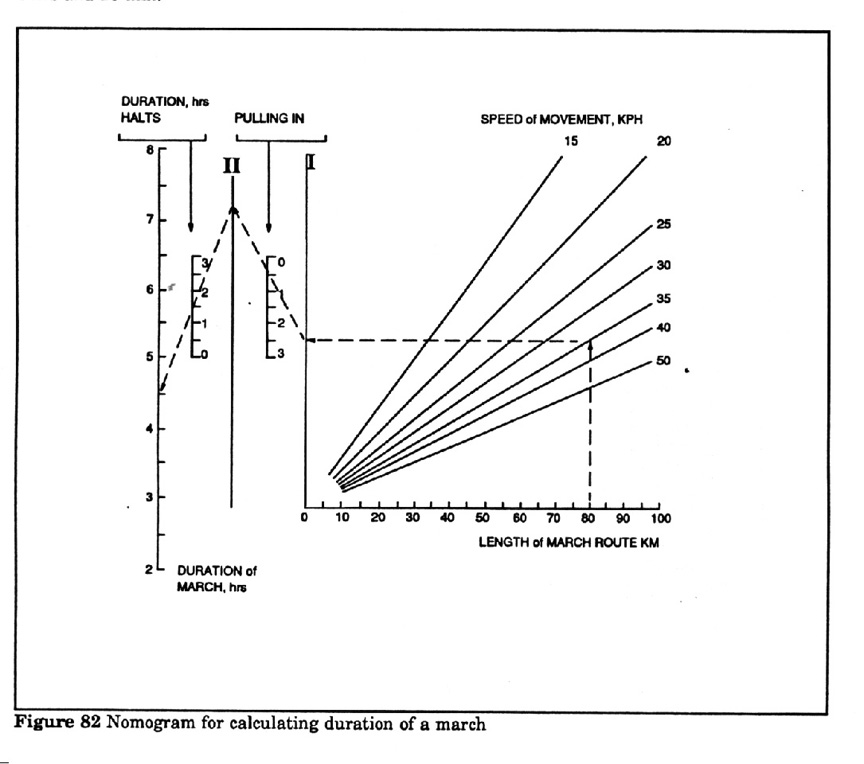
Example problem using nomogram: Calculate the duration of a move along a 80
km route with an average speed of 35 km/hr, duration of halts total 1 hr &
30 min, and time taken to deploy into new area is 30 min.
Solution: Start at the 80 point on the bottom scale "Length of
March" go up to the "Speed of movement -35 kph" line then
horizontally across to the I line. Draw a line from that point to the II line
passing through the .5 point on the "Pulling in" line, then another
line downwards from the II line passing through 1.5 on the "Duration of
halts" line. This intersects the "Duration of march" line at 4
hrs and 20 min.
|
|
| |
Figure 82 - Nomogram for calculating duration
of a march
|
|
| |
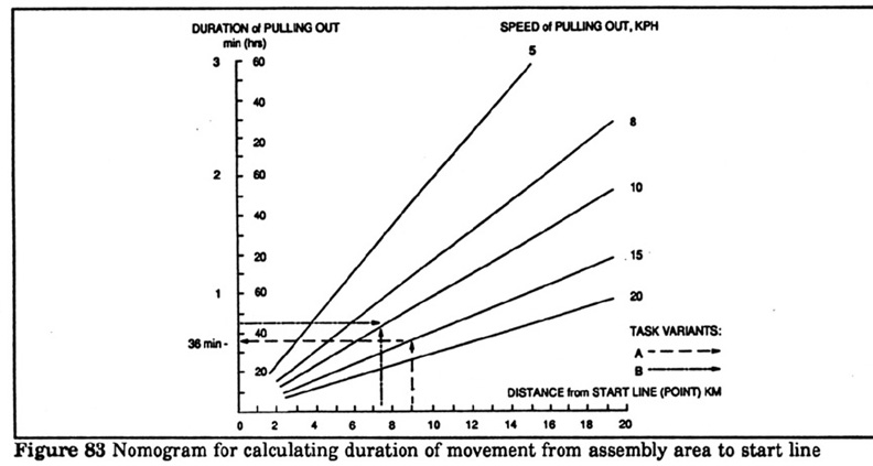
(2) Calculation of Time to Begin Move
to Start Line:
This calculation is used to determine when a unit should begin moving out of
its assembly area in order for the head of the column to cross the start line
(SL) at the prescribed time. The given data are the distance from the assembly
area to the start line and the rate of march.
The formula is:
 where:
Dn=distance to SL; \
tN=time column starts to move;
Vv=rate of movement to SL;
60=conversion factor Hr to min;
T=time head of column passes SL;
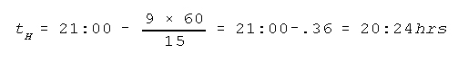
Example problem: Determine the starting time for a column when the time for
the head of the column to pass the start line is planned for 2100 hrs, the
distance to the start line is 9 km, and the rate of march while moving out is
15 kph.
Solution:
|
|
| |
Example using nomogram (Figure
83):
|
|
| |
Using the same initial data as the previous
example enter the nomogram on the X axis at 9 km move up to 15 kph line then
across to the 36 min on the Y axis.
Example 2: Calculate the required speed of movement for the column to reach the
start line with a distance of 7.5 km and a time of 45 min.
Solution: Draw lines from the 7.5 km and 45 min points on the scale. These
intersect on the 10 kph line.
|
|
| |
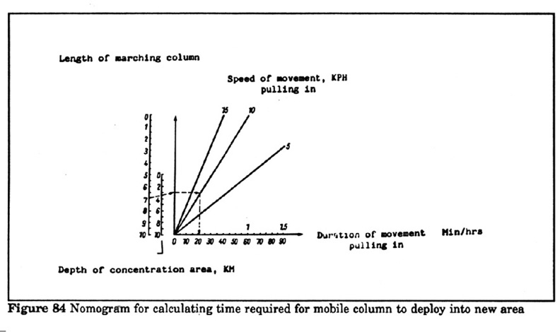
(3) Calculation of Time to Deploy
into a New Assembly Area:
As noted in formula (1), this only must be calculated when the depth of the new
area is less than the length of the mobile column. This is because in this case
the head of the column will have stopped at the far end before the tail reaches
the near side of the area. The formula gives the time it takes to deploy, once
the head of the column has reached the new area.
|
|
| |
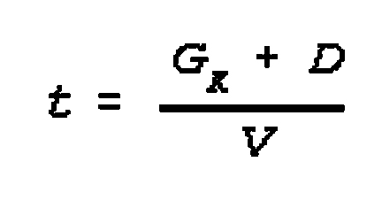
The formula is:
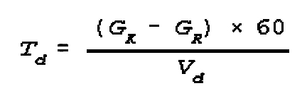
Td=time for deployment;
GK=length of column;
GR=depth of area;
Vd=speed during deployment;
60=convert hr to min;
Example problem: Calculate the time required for a column to occupy a new
area if the length of the column is 7 km, the depth of the new area is 3.5 km
and the speed of movement during deployment is 10 kph.
Solution:=(7 - 3.5) x 60=0.35 x 60=21 Min 10
Using the nomogram (Figure 84) provides the same answer. Enter at 7 on the
length of column scale cross 3.5 on the depth of area scale then horizontally
to 10 kph and then down to 21 min on the duration of movement scale.
|
|
| |
Figure 84 - Nomogram for calculating time required for moble
column to deploy into new area
|
|
| |
(4) Calculation of Time a Unit will
be in a New Area
This calculation combines the previous formulas in order to determine the clock
time a unit will be deployed in the new area. It takes into consideration the
time required for a unit to deploy into an area when the depth of that area is
less than the length of the marching column. It also includes time for halts en
route.
Formula of calculation:
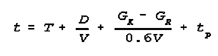
where:
t=clock time a unit will be regrouped in new area in hrs;
T=time (astronomical) of passing start point (line) by front of column in
hrs/mins;
D=length of route and distance away of new concentration area in km;
V=average speed of movement;
GK=length of column;
GR=depth of new concentration area in km (considered only when the
depth is less than the length of column);
0.6=coefficient, which takes into account the lowering of the average march
speed while deploying into the new assembly area.
tp=duration of halts en route in hrs.
|
|
|
This calculation may be conveniently
performed by entering the data into the table provided.
Figure 85 - Form to calculate time unit is in new area
CALCULATION OF TIME UNIT IS ASSEMBLED IN NEW AREA
|
| No |
Initial data and values to be
calculated |
Units |
Calculation variant |
Remarks |
| Example |
2 |
3 |
4 |
| 1 |
Length of march route |
km |
167 |
|
|
|
|
| 2 |
Average rate of movement |
|
18 |
|
|
|
|
| 3 |
Length of moving column |
|
7.5 |
|
|
|
|
| 4 |
Depth of new assembly area |
|
4 |
|
|
|
|
| 5 |
Duration of halts |
|
1.5 |
|
|
|
|
| 6 |
Time of passing start line (SL) |
|
10.0 |
|
|
|
|
| 7 |
(1) ÷ (2) |
|
9.3 |
|
|
|
|
| 8 |
(3) - (4) |
0.1 |
3.5 |
|
|
|
|
| 9 |
(2) x 0.6 |
0.1 |
10.8 |
|
|
|
|
| 10 |
(8) ÷ (9) |
0.1 |
0.3 |
|
|
|
|
| 11 |
Overall duration of march (5) + (7) +
(10)
|
0.1 |
11.1 |
|
|
|
|
| 12 |
Time unit is concentrated in new area (6) + (11) |
hrs |
21:06 |
|
|
|
|
|
|
| |
(5) Calculation of the Duration of a
March from one Area to Another
This is a more sophisticated version of the basic march formula to take account
of possible reductions in the capacity of the road or other influences on the
achievable rate of movement of the columns.
The formula is:
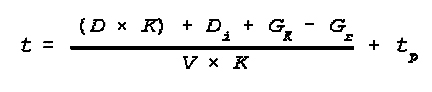
when GK > Gr
where:
t=duration of march in hours;
D=length of march in km;
K=coefficient for reduction in average rate of march of moving columns during
entering and leaving the route of march;
Di=distance of start point from original assembly area in km;
GK=depth of column in km;
Gr=depth of the new assembly area in km;
V=average rate of movement of column in km/hr;
tp=duration of halts or delays during movement in hrs.
Example problem: Determine the duration of march for a column 11.2 km long
to a new area at a distance of 87 km. The start point is 4.5 km from the
original assembly area and the depth of the new area is 7 km. The average rate
of march is 18 kph with a coefficient of reduction of speed of 0.6. There will
be a total of 1 hr of halts.
Answer is 6 hr 38 min.
|
|
| |
Figure 86 - Form to calculate duration of march
TABLE FOR CALCULATING DURATION OF A MARCH
|
| No |
Initial data and values to be
determined |
Units |
Calculation variant |
Remarks |
| Example |
2 |
3 |
| 1 |
Route length |
km |
87 |
|
|
|
| 2 |
Speed reduction factor |
-- |
0.6 |
|
|
(1) x (2) |
| 3 |
Distance to start point |
km |
4.5 |
|
|
+ (3) |
| 4 |
Column depth |
km |
11.2 |
|
|
+ (4) |
| 5 |
Depth of new concentration region |
km |
7 |
|
|
- (5) |
| 6 |
Rate of march |
km/hr |
18 |
|
|
÷ (6) |
| 7 |
Speed reduction factor |
-- |
0.6 |
|
|
÷ (7) |
| 8 |
Length of halts |
hr |
1 |
|
|
+ (8) |
| 9 |
March duration |
hr |
6.64 |
|
|
=ans |
|
|
| |
(6) Determine the Required Movement
Rate for a Unit to Regroup in a New Area.
This is a more elaborate version of the basic movement formulas to take into
account more variables and possible interactions during the movement.
The formula is:

|
|
| |
Example problem: Determine the required rate
of march if a column has a depth of 8.7 km and the time allowed to assemble in
the new area 5.5 km deep is 6 hours. The distance to the new area is 128 km and
to the start point is 6 km. The coefficient for reduction of rate is .7 and the
duration of planned delays is 45 min.
Answer is 27 kph.
|
|
| |
Figure 87 Form to calculate required rate of
travel
FORM FOR CALCULATING REQUIRED TRAVEL SPEED
|
| No |
Initial data and values to be
determined |
Units |
Calculation variant |
Remarks |
| Example |
2 |
3 |
| 1 |
Route length |
km |
128 |
|
|
|
| 2 |
Speed reduction factor |
-- |
0.7 |
|
|
|
| 3 |
Distance to start point |
km |
4.5 |
|
|
|
| 4 |
Column depth |
km |
8.7 |
|
|
|
| 5 |
Depth of concentration area |
km |
5.5 |
|
|
|
| 6 |
Maximum travel time allowed |
hr |
6 |
|
|
|
| 7 |
Halt time |
hr |
0.75 |
|
|
|
| 8 |
Speed reduction factor |
-- |
0.7 |
|
|
|
| 9 |
Required travel speed |
km/hr |
27 |
|
|
|
|
|
| |
(7) Calculation of Length of Route,
Average speed and Duration of Movement of Moving Column
This calculation combines the basic equations. It is used when the total
distance to be traveled is composed of segments having different route
characteristics. The different characteristics result in different possible
movement rates over the individual sectors. The initial data is the length of
each sector, the movement rate over each sector, the length of the column and
the depth of the new assembly area. Formulas for calculation:
|
|
| |
where:
 D=length of route in km; \
Li=length of each sector of different types of road each allowing
Vi speed of movement of columns in km;
td=overall time on the route in hrs;
Vi=speed of movement on a type of sector of the route in kph;
V=average speed of movement in kph.
GK=length of column in km;
GP=depth of concentration area in km;
0.6=coefficient of reduction in speed of the column while deploying into the
new area or depending on local conditions;
tn=overall time of halts.
|
|
| |
Figure 88 - Form for calculation of duration
of march over complex route
CALCULATION OF TRANSIT TIME OVER MULTI-SEGMENT ROUTE
|
| No |
Initial data - form of
calculations |
Units |
Calculation variants |
Remarks |
| Example |
2 |
3 |
| 1 |
Length of paved roads |
km |
42 |
|
|
|
| 2 |
Speed of movement on 1 |
km/hr |
35 |
|
|
|
| 3 |
Length of improved dirt roads |
km |
18 |
|
|
|
| 4 |
Speed of movement on 3 |
km/hr |
25 |
|
|
|
| 5 |
Length of dirt roads |
km |
21 |
|
|
|
| 6 |
Speed of movement on 5 |
km/hr |
15 |
|
|
|
| 7 |
Length of field tracks |
km |
8 |
|
|
|
| 8 |
Speed of movement on 7 |
km/hr |
10 |
|
|
|
| 9 |
Length of moving column |
km |
6.8 |
|
|
|
| 10 |
Depth of new assembly area |
km |
3 |
|
|
|
| 11 |
Overall time for halts |
hr |
1.5 |
|
|
|
| 12 |
Total length of route (1) + (2) + (5) +
(7)
|
km |
89 |
|
|
|
| 13 |
(1) ÷ (2) |
|
1.2 |
|
|
|
| 14 |
(3) ÷ ((4) |
|
.7 |
|
|
|
| 15 |
(5) ÷ (6) |
|
1.4 |
|
|
|
| 16 |
(7) ÷ (8) |
|
0.8 |
|
|
|
| 17 |
Time of movement (13) + (14) + (15) +
(16)
|
hr |
4.1 |
|
|
|
| 18 |
Average speed (12) ÷ (17) |
km/hr |
22 |
|
|
|
| 19 |
(9) - (10) ÷ [0.6 x (18)] |
|
3.8 |
|
|
|
| 20 |
Time of deploy - new area (19) ÷ [0.6 x
(18)]
|
hr |
.3 |
|
|
|
| 21 |
Duration of move (11) + (17) + (20)
|
|
5.9 |
|
|
|
|
|
| |
(8) Calculation of Overall Depth of
Column Consisting of Several Sub-columns:
This technique is for calculating the total length of a moving formation on a
route given the number of vehicles in the moving columns and the distances
between them is known. It is also used to determine the required distances
between vehicles.
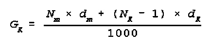
The formula is:
where:
Gk=formation depth in km;
Nm=number of vehicles;
dm=distance between vehicles;
NK=number of columns;
dK=distance between columns;
1000=convert meter to km.
Example problem: Determine the length of a moving formation consisting of four
columns, if the overall number of vehicles is 169, distance between columns is
600 meters, and distance between vehicles is 40 meters.
Solution:

|
|
| |
Figure 89 - Example using the
nomogram :
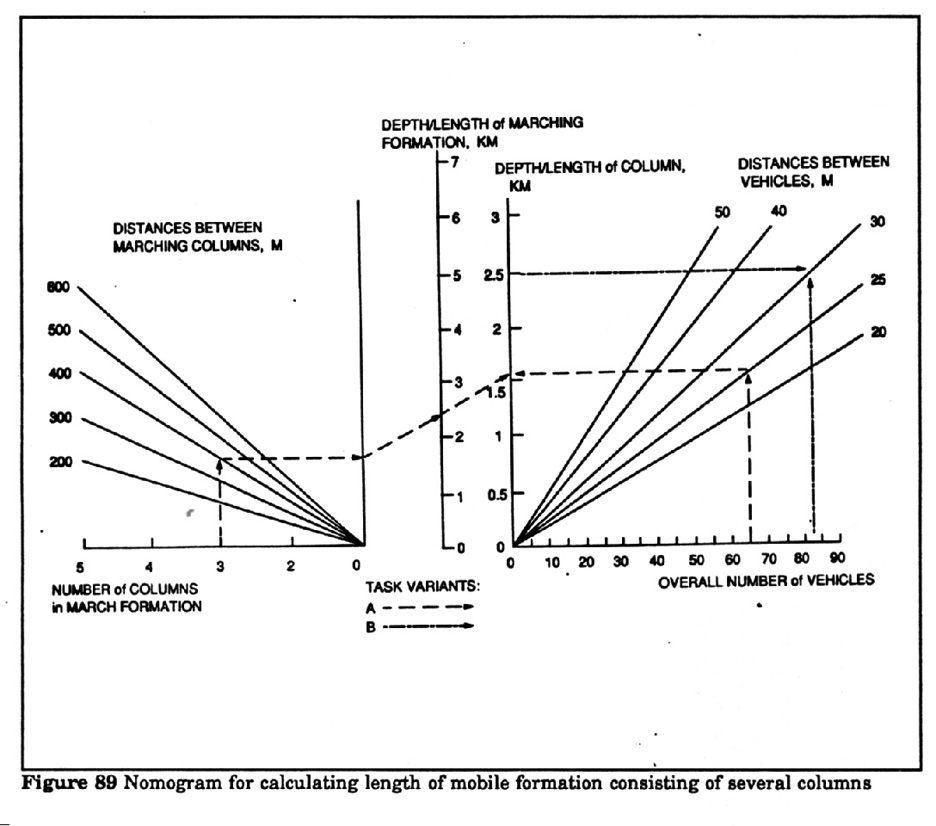
Determine the length of a moving formation if there are 3 moving columns
and the distances between them is 400 meters, the overall number of vehicles is
65, distance between vehicles is 25 meters (variant a).
Solution: First find the column depth without considering the distances between
col use the right side of the nomogram and draw a perpendicular line from the
"65" mark on the "Total number of vehicles" scale to the
intersection with the "distances between vehicles- 25" line; from
this point draw a horizontal line to the intersection with the "Column
depth" scale. In the left part of the nomogram from the "3" mark
on the "Number of columns in route formation" scale draw a
perpendicular line to the intersection with the "Distances between
columns- 400" line, from this point draw a horizontal line to the unnamed
scale. Then connect the two obtained marks and find the calculation result on
the "Depth of marching formation scale.
Answer: is 2.5 km.
Example variant b: Determine the required distances in a column consisting
of 83 vehicles given that the length of the column must not exceed 2.5 km.
Solution: On the nomogram draw a horizontal line from the "2.5"
mark on the "Depth of column" scale. Then from the "83"
mark on the overall number of vehicles" scale draw a perpendicular line
and at the intersection of these lines read the required distances between the
vehicles. The answer is 30 meters.
|
|
| |
Figure 89 - Nomogram to
calculate the lenfth of mobile formation consisting of several columns on march
|
|
| |
(9) Calculation of Duration of
Passage of Narrow Points and Difficult Segments
This calculation is the basic one for determining the time it will take a
column of given length to pass through a constriction in the route. It does not
take into consideration the issue of vehicle bunching up at the halt before the
constriction nor the time to regain column vehicle separation distances after
the passage. Therefore more elaborate formulas are used to determine the
overall effect of a constriction on a full march.
|
|
| |
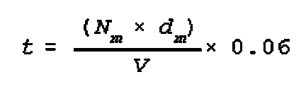
The formula for short obstacles is:
where:
Nm=number of vehicles;
dm=distance between vehicles;
t=time required to overcome obstacle in minutes;
V=speed of column through obstacle;
0.06=conversion factor km/hr to meters/min.
Example Calculation (A): Calculate the time required to cross an obstacle by a
column of 54 vehicles with distance between vehicles of 75 meters and a maximum
speed of 10 kph.
t=(54 x 75) x 0.06 ÷ 10=24 Min
|
|
| |
There are two types of difficult sections on
routes; the first is minor ones whose length is less than the marching column,
and the second is major obstacles with length greater than the length of the
column. The main factor for shorter obstacles is the number of vehicles in the
column, the distances between them and their speed of movement while passing
the obstacle. The main data for the larger obstacles are the length of the
column, the length of the sector and the speed of movement.
The formula for major obstacles:
where:
Gk=length of column;
D=length negotiated segment;
t=duration to overcome obstacle in hours;
v=speed through obstacle.
Example calculation (B): Determine the time for a column 2.5 km long to pass
through an obstacle 5.5 km long at a movement rate of 15 km per hr.
(2.5 + 5.5) ÷ 15=8 ÷ 15=0.53=32 min
Example calculation (C): Determine what length of column can negotiate a pass
2.5 km long at a speed of 8 kph in a 45 min. Gk=(V x t) - d=(8 x
0.75) - 2.5=3.5 Km
Solution: 3.5 km
Example using nomogram (Figure 90):
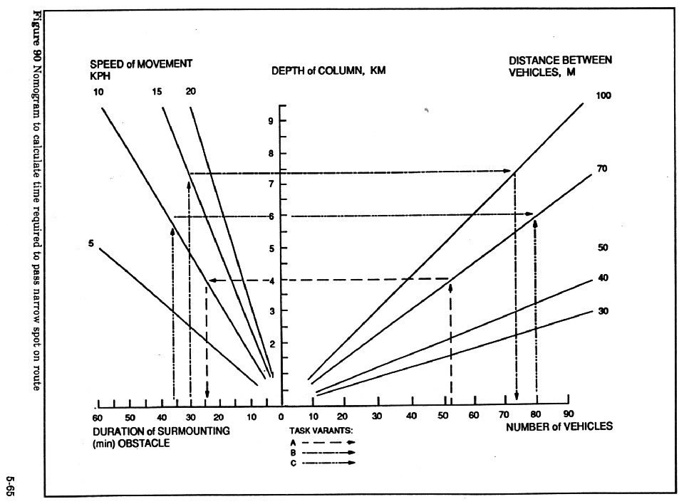
Example calculation: Using data from example (A), start at 54 on
"Number of vehicles" line and draw a perpendicular to the
intersection with the "Distances between vehicles - 74" line. From
that point draw a horizontal line to the intersection with the "Travel
speed - 10" line. From this point drop a perpendicular line to the
"Duration of surmounting obstacle" scale at which point the result
shows 24 minutes.
Example calculation variant B: Determine the number of vehicles able to cross
an obstacle within 30 min, if the allowable movement speed is not more than 15
km per hr and the distance between vehicles is 100 m.
Solution: Start at 30 on "Duration of surmounting obstacle" scale,
move vertically to "15 km per hr on speed" scale, then horizontally
to "Distance between vehicles -100 m" and down to "Number of
vehicles" scale where the result shows 75 vehicles.
Example calculation variant C: Calculate the distance between vehicles in a
column of 80 vehicles in order that the column crosses a bridge within 36 min
at rate not more than 10 kph.
Solution: Starting at 80 on the "Number of vehicles" scale and at 35
min on the "Duration of surmounting obstacle" scale draw
perpendicular lines. From the intersection of the perpendicular with the
"Speed of movement -10" scale draw a horizontal line to intersect
with the first perpendicular. The point of intersection is on the
"distance between vehicles- 75" line. This means that the distance
between vehicles must be no more than 75 meters.
|
|
| |
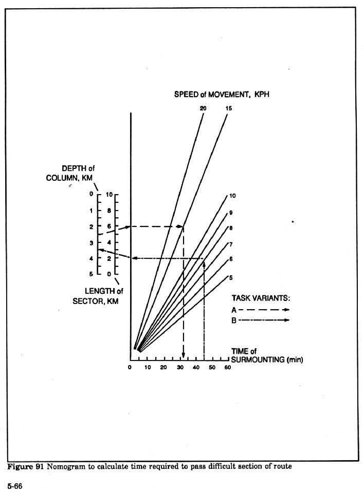
Figure 91 - Nomogram to
calculate time required to pass difficult section of rooute:
 |
|
| |
Example calculation variant A: Determine the
time required to pass through a damaged strip of road, if the length of the
sector is 5.5 km, the length of the column is 2.5 km, and the average speed
while crossing the sector is 15 kph.
Solution: Mark on the "Depth of column" scale at 2.5 and the
"Length of sector" scale at 5.5 and then draw a line through these
points to the intersection with the Y or vertical axis. From this point draw a
horizontal line to the "Speed of movement - 15" line and draw a
perpendicular down to the "Time of surmounting" line to read the
result of 32 min.
Example calculation variant B: Determine what length of column can negotiate a
pass 2.5 km long at speed of 8 km per hr in a given time.
Solution: From the 45 mark on the "Time of surmounting" scale draw a
perpendicular to the intersection with the "Speed of movement- 8"
line. From this point draw a horizontal line to the Y axis. Connect this point
with the 2.5 mark on the "Length of sector" line and continue it to
intersect with the "Depth of column" line. This shows the result is
3.5 km. This means that a column of 3.5 km length may negotiate the passage in
the given time.
|
|
| |
(10) Calculation for
Passage Times Across Start Point (SL) by the Head and Tail of the Column
This calculation also determines the time for a column to pass a given point,
however, since there is no delay as with an obstacle, the time interval is
governed by the length of the column and its velocity. Since we are not
interested in the length of time the column requires, but the clock times the
head and tail cross, the equations yield time in military time.
The formula is:
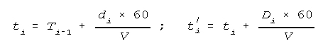 where:
ti=SL crossing time of the head of the march column i in hours and minutes;
Ti-1=the time for passing the line by the tail of the leading march
column in hours and minutes; for the head of the first column this time is the
time specified for passing the line by the head of the entire formation, for
instance, by the column of the leading unit on a route;
di=the specified distance between the lead and the i march column in
km;
60=factor for converting hours into minutes;
V=average speed in km per hr;
t'i=the time for passing the line by the tail of the i route column
in hours and minutes;
Di=depth of the i column in km.
Example: to determine the passage time of the starting line or other regulation
point by the head and tail of the third column in a formation, when the passage
time of the cited point by the tail of the previous column is 21:15, the
established distance between the columns in 1.5 km, the depth of the column is
1.8 km and the movement speed is 25 km per hr.
solution:
t3=21:15 + [(1.5) x (60)} ÷ 25=21:15 + 0.04=21:19;
t'3=21:19=1.8 x 60 ÷ 25=21:19=0.04=21:23;
this means the third column in the march formation will pass the regulation
point with its lead at 21:19 and its tail at 21:23 hrs.
Example calculation using the nomogram Figure 92: The nomogram may be used to
speed up the calculation of the passage of a line by the head and tail of the
column. To determine the passage time of an initial line by the head and tail
of a march column 7 km line with the condition that the time for crossing the
line by the tail of the lead column is 20:20, the distance between the columns
is 5.5 km and the travel speed is 25 km per hr.
Solution: Draw a perpendicular line up from the horizontal axis, "Depth of
column or distance between columns" scale from the 5.5 mark to the
intersection with the "Average speed of columns -25" line. From this
point draw horizontal line to the "Time of passing point" scale and
read the result=13.3 or approximately 13 minutes. This is the time in which the
head of the stated column must pass the point after it is passed by the
previous column (at 20:00). The time for passing a point by the tail of a
stated column is solved in a similar manner. For this draw a perpendicular line
from the 7 mark on the "Depth of column axis" to the intersection
with the "Average travel speed line - 25". From this point draw a
horizontal line to the "Time of passing point" scale and read the
result of 17 minutes. This means that this column must pass the control point
with its tail at 20:30.
|
|
| |
Figure 92 Nomogram to calculate
the front and tail of a column will pass a specific location.
|
|
| |
|
|
| |
(11) Calculation of Expected Time and
Distance of Probable Point of Contact with Advancing Enemy
Clearly this is one of the most important calculations Soviet commander's make
regularly during the course of combat. As the discussion of meeting engagements
in Chapters One and Two indicates, the commander's effort to control the flow
of battle focuses heavily on the relative times and place of introduction of
his second echelon versus the enemy's reserves, both of which are moving
forward.
The formula is:
 where:
te=expected tome of meeting in hours;
D=initial distance between opposing groupings in km;
Vf=movement rate of friendly troops in km per hr;
Ve=movement rate of enemy forces in km per hr;
dl=distance from friendly initial position to expected point of
contact in km;
Example calculation: Determine the expected time of meeting and distance to
probable encounter line when enemy is located 63 km away, his average forward
speed is 25 km per hr, and average speed of friendly troops is 20 km per hr.
Solution: the equation yields distance of 28 km and time of 1 hr and 24 min.
Example using nomogram Figure 93: Determine the expected time of meeting and
distance to line of contact with enemy if at 18:00 the advancing enemy is
located at a distance of 64 km, his average speed is 15 km per hr, and friendly
troops are moving at 20 km per hr.
To use nomogram (variant a) find the marks "20" and "15" on
the "Speed of movement of own forces" and "Speed of movement of
enemy" lines respectively, draw a line through these points to
intersection with horizontal scale and read mark of 35. Then move downward
along the line shown by the dots to the intersection with the perpendicular
established from the "64" mark on the "Distance between our own
and enemy forces" scale. From this point of intersection draw a horizontal
line to the "Anticipated time of meeting" scale and read the
calculation result of 1 hr and 50 min. This will be the length of time from the
start time to meet the enemy. That means 18:00 plus 1:50 gives 19:50.
To determine the distance of the probable meeting line with the enemy (variant
b) from the result of 1 hr 50 min, draw a horizontal line to the intersection
with the speed line (ie at mark 20), which corresponds to the travel speed of
the friendly troops. From the obtained point, drop a perpendicular line to the
"Distance between friendly and enemy forces" scale and read the
calculation result of 36 km.
|
|
| |
Figure 93 Nomogram to
calculate the time anddistance to point of a meeting engagement
 |
|
| |
(12) Calculation of Time Required for
Advancing and Deploying Sub-units to Change From Line of March into the
Attack
Determination of the time a unit should begin to move for the advance from its
assembly area to the line of commitment into battle and assault on the enemy
position is a complex application of the basic time and distance formula. All
times are measured backwards from "CHE" hour, the moment the troops
hit the first line of the defending enemy's position. The total time from
beginning of movement in the assembly area is composed of the segments of time
while moving in each type of deployment, that is: line of attack, company
column, battalion column, and regimental column. It also includes the time it
takes to shift from one formation to the other and any time for halts and
delays en route. This is one of the most important and fundamental of tactical
calculations. The times for sub-unit movement are tied exactly into the times
for the artillery preparatory fire and air strikes.
The required given data are the distances between each of the deployment
and regulating lines, distance of the attack line from the enemy's forward line
of defense, distance of the start line from the unit assembly area, the average
speed of movement while mounted in the columns, the coefficient for speed
reduction during deployment actions, the speed of movement in attack formation,
the depth of the columns, and distance between first and second echelons of the
units. The set of formulas are:


t'i=ti - (Gk + dk) x (90)/ V
where:
ta=time for crossing final deployment into line of attack -
"Che" hour -in minutes;
Da=distance of line for going into attack formation from the forward
edge of the enemy position in km;
Va=rate of movement in attack formation in kph;
tr=time for crossing the line of deployment into company columns at
("Che" - minutes)
Dr=distance of line of deployment into company columns from the line
of deployment into attack formation in km;
V=average rate of movement of subunits in mounted formation during march;
tb=time for crossing line of deployment into battalion columns at
("Che" - minutes);
Db=distance of line for deployment into battalion columns from line
of deployment into company columns in km;
trr=time for crossing the last regulation line or point prior to the
deployment into battalion columns;
Drr=distance of last regulation line from the line for deployment
into battalion columns;
ti=time for passing the start line at ("Che" - minutes)
Di=distance of start line from last regulating line in km;
tvit=time to begin movement of subunits in assembly area;
D=distance of start line from the last unit assembly area;
t'i=time for crossing the start line by the 2nd echelon
of units at ("Che" - minutes);
Gk=depth of the mounted column of first echelon of units in km;
dk=distance between the tail of the first echelon and head of the
2nd echelon of the units in km;
The numbers 60 and 90 are coefficients for conversion of time in minutes for
the average speed of movement during the deployment of the units at each of the
lines. For example, the 90 shows that the average maneuver speed of the unit
during the actual deployment on a line decreases by a factor of 1.5 in
comparison with the speed of forward movement between the lines. Depending on
the concrete conditions and situation for movement on the terrain, this could
be some other factor.
To perform the calculation the required data may be entered into the table. The
result will be the planning data for start of forward movement and deployment
times for each shift of sub-unit columns. Since all times are measured backward
from "Che", the planner must remember to subtract the values
indicated in lines 12, 15, 18, 21, 24, and 27 from Che; and add the value for
time in line 30 to the time in 24 to obtain line 31.
|
|
| |
Figure 94 Calculation of time to adevance and deploy sub-units for shift
into attack from line of march
CALCULATION OF TIME TO ADVANCE AND DEPLOY SUB-UNITS
FOR SHIFT INTO ATTACK FROM LINE OF MARCH
|
| No |
Initial data, values and calculations to
perform |
Units Precision |
Calculation variant |
| 1 |
2 |
3 |
| 1 |
2 |
3 |
4 |
5 |
6 |
| 1 |
Distance of attack line from enemy front line |
|
|
|
|
| 2 |
Distance of line to deploy into company columns from attack
line |
|
|
|
|
| 3 |
Distance of line to deploy into battalion columns from line of
company columns |
|
|
|
|
| 4 |
Distance of regulation line from line to deploy into battalion
columns |
|
|
|
|
| 5 |
Distance of regulation line from start line |
|
|
|
|
| 6 |
Distance of start line from the unit assembly (FUP)
area |
|
|
|
|
| 7 |
Movement speed into the attack |
|
|
|
|
| 8 |
Average speed during march |
|
|
|
|
| 9 |
Dept of first echelon march column |
|
|
|
|
| 10 |
Interval between first and second echelon columns |
|
|
|
|
| 11 |
(1) x 60 |
|
|
|
|
| 12 |
Time to cross line for shifting to attack (Che - min)
(11) ÷ (7)
|
|
|
|
|
| 13 |
(2) x 90 |
|
|
|
|
| 14 |
(13) ÷ (8) |
|
|
|
|
| 15 |
Time to cross line of deployment into company columns: (Ch - ) (12)
+ (14) |
|
|
|
|
| 16 |
(3) x 60 |
|
|
|
|
| 17 |
(16) ÷ (8) |
|
|
|
|
| 18 |
Time to cross line of deployment into battalion columns: (Ch - )
(15) + (17) |
|
|
|
|
| 19 |
(4) x 60 |
|
|
|
|
| 20 |
(19) ÷ (8) |
|
|
|
|
| 21 |
Time to cross regulation line (Ch - ) (18) +
20)
|
|
|
|
|
| 22 |
(5) x 60 |
|
|
|
|
| 23 |
(22) ÷ (8) |
|
|
|
|
| 24 |
Time to cross start line (Ch - ) (21) + (23) |
|
|
|
|
| 25 |
(6) x 90 |
|
|
|
|
| 26 |
(25) ÷ (8) |
|
|
|
|
| 27 |
Time to start moving out of assembly area - 1st echelon (Ch - )
(24) + (26) |
|
|
|
|
| 28 |
(9) + (10) |
|
|
|
|
| 29 |
(28) x 90 |
|
|
|
|
| 30 |
(29) ÷ (8) |
|
|
|
|
| 31 |
Time for second echelon to pass start line (SL) (Ch - ) (24) -
(30) |
|
|
|
|
|
|
| |
(13) Calculation of the Time and
Distance to the Line of Contact
This method takes into consideration the many situational factors that are
ignored in the simpler formula and nomogram. In fact, there are so many
possible influences on the time the two sides will meet and hence the location
of meeting that a nomogram can only give a crude approximation of the answer.
With the use of computers or even hand calculators and an established procedure
such as that shown in this table it is possible to assess the influence of many
more factors.
The set of formulas is:
tv={D + [(tn x Vn) + (tp x
Vp)]} ÷ (Vn + Vp)
Tn=t1 + t2 t3;
TP=t1' + t2' + t3'
where:
tv=expected time if contact with enemy in hours;
D=distance between forces of the two sides in km;
tn=total delay time for own force in hrs;
Vn=speed movement of own forces in km per hr;
tp=total delay time of enemy in hrs;
Vp=speed movement of enemy in km per hr;
lp=distance to expected line of meeting with enemy;
t1 (t'1)=delay - (time difference) start of
movement of one side versus other in hrs;
t2 (t'2=duration of halts of forces of each
side in hrs;
t3 (t'3)=duration of delay of forces due to
strikes by opponent en route in hrs;
Astronomical time of meeting enemy depends on complex conditions. Determine it
by adding the relative time obtained as a result of the calculation with the
astronomical time of the beginning of the approach of the opposing forces.
For example if the time to start march of own forces is 9PM the starting time
for the enemy is 10PM then astronomical time to start the approach is 9PM. If
the calculated time for meeting is about 2.5 hours then the time for meeting
would be 11:30.
Example problem: determine the expected time of meeting and the distance to
likely line of contact with the enemy and the duration of movement to that line
under following conditions:
----- start time of own forces - 20:00 hrs;
----- start time of enemy forces - 21:00 hrs;
----- distance to enemy - 105 km;
The commander decides there will be a break of 20 minutes (.3) hr during the
advance. The plan is to delay enemy forces 30 -40 minutes (.6) hr. It is
assumed that during movement enemy will be required to take halts of 30 minutes
(0.5) hrs. The speed of movement of own forces is 28 km per hr. The speed of
movement of the enemy is 19 km per hr.
The answer is that contact will be at 11:20 at a distance of 84 km. Duration of
movement to meeting line is 3 hrs.
|
|
| |
Figure 95 Form for calculation of expected
time and location of meeting engagement
CALCULATION OF EXPECTED TIME AND DISTANCE
TO PROBABLE LINE OF MEETING ENGAGEMENT
|
| No |
Initial data, values and
calculations |
Units Precision |
Calculation variant |
| Example |
2 |
3 |
| 1 |
2 |
3 |
4 |
5 |
6 |
| 1 |
Friendly force starts advance |
hr, min |
20:00 |
|
|
| 2 |
Enemy force starts advance |
hr, min |
21:00 |
|
|
| 3 |
Distance between opponents at start |
km (1.0) |
105 |
|
|
| 4 |
Delay in advance of friendly relative to enemy |
hr (0.1) if 1 > 2
|
-- |
|
|
| 5 |
Total duration of halts of friendly |
hr (0.1) |
0.3 |
|
|
| 6 |
Total duration of delays of friendly by enemy |
hr (0.1) |
-- |
|
|
| 7 |
Friendly force travel speed |
km/hr (1.0) |
28 |
|
|
| 8 |
Delay of enemy start relative to friendly |
hr (0.1) if 2 > 1
|
1 |
|
|
| 9 |
Total duration of halts of enemy |
hr (0.1) |
0.5 |
|
|
| 10 |
Total duration of delays of enemy due to friendly |
hr (0.1) |
0.6 |
|
|
| 11 |
Enemy force travel speed |
km/hr (1.0) |
19 |
|
|
| 12 |
(4) + (5) + (6) |
(0.1) |
0.3 |
|
|
| 13 |
(12) x (7) |
(0.1) |
8.4 |
|
|
| 14 |
(8) + (9) + (10) |
(1.0) |
2.1 |
|
|
| 15 |
(14) x (11) |
(1.0) |
40 |
|
|
| 16 |
(3) + (13) + (15) |
(1.0) |
153 |
|
|
| 17 |
(7) + (11) |
(0.1) |
47 |
|
|
| 18 |
Expected time of meeting (relative) (16) ÷
(17)
|
hr (0.1) |
3.3 |
|
|
| 19 |
Duration of travel time to meeting line: (18) - (12) |
hr (0.1) |
3 |
|
|
| 20 |
Distance to meeting line: (19) x (7)
|
km (1.0) |
84 |
|
|
|
|
| |
(14) Calculation of Expected Time and
Rate of Overtaking when Pursuing the Enemy:
Naturally the commander hopes to use this calculation often! The initial data
are the distance between the enemy and friendly forces, the average travel
speed of friendly and enemy forces, or the ordered time to overtake him.
 where:
to=time to overtake enemy in hours;
D=distance to the enemy in km;
Vn=friendly speed in pursuit in km per hr;
Vp=enemy speed in retreat in km per hr;
Example: Determine how much time it will take for forces to overtake a
retreating enemy when the distance to him is 20 km, his rate of retreat is 10
km per hr, and the rate of advance of friendly forces is 25 km per hr.
Solution: to=20 ÷ (25 - 10)=1.3 hrs ;
Determine the pursuit speed required to enable friendly forces to overtake
enemy in 45 min, when he is 15 km away and his travel speed is 12 km per hr.
Solution: Vn=((15 + 0.75) (12)) ÷0.75=32 km per hr.
Examples of calculations using the nomogram Figure 96:
Determine the expected time to overtake enemy when his distance is 30 km, his
travel speed is 20 km per hr, and the speed of pursuit is 28 km per hr. In the
calculation (variant a) establish a perpendicular line from the "30"
mark on the "Distance between friendly and enemy forces" scale. Then
draw a line through the "28" mark on the "Friendly forces travel
speed" and the "20" mark on the "Enemy travel speed"
scale to its intersection with the horizontal upper axis. From this point draw
a line down as shown by the dots to the intersection with the previously set
perpendicular line. From the point of intersection draw a horizontal line to
the right and read off the result of 3 hrs and 45 min on the "Expected
encounter time" scale.
Determine the required pursuit speed to intercept the enemy in 1 hr and 20 min,
when the enemy is at a distance of 40 km and is traveling at a speed of 5 km
per hr.
In calculation (variant b) establish a perpendicular line from the
"40" mark on the "Distance between friendly and enemy
forces" scale to the intersection with the horizontal line, drawn from the
1 hr and 20 min mark on the "Expected encounter time" scale. From the
meeting point draw a line, as shown by the dots and dashes, to the horizontal
scale. Draw a line through the point of intersection of this scale and the 5
mark on the "Enemy travel speed" scale and continue it to the
intersection with the "Friendly force travel speed" scale, where the
result is 35 km per hr. This means that the pursuit speed must he at least 35
km per hr.
|
|
| |
Figure 96 Nomogram for
calculating expected time and speed to overtake retreeating enemy
 |
|
| |
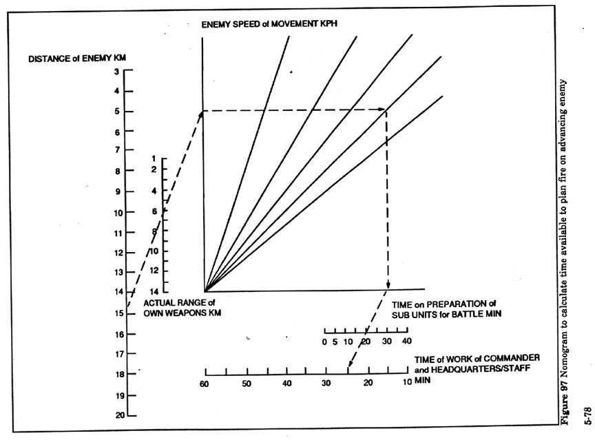
(15) Calculation of the Work Time
Available to the Commander and Staff for Organizing Repulse of Advancing Enemy
Forces:
This is obviously a critical issue in meeting engagements and encounter battle.
It is also relevant to defensive situations when preparing fire on the
attacker. The method is designed to determine the time the commander and staff
will have to organize the enemy's defeat by firing on the advancing forces
relative to the distance to the enemy, the speed of his advance, the effective
range of friendly weapons and the time required to prepare the sub-units to
fire. In this example it is assumed that the enemy will be taken under fire
beginning at the maximum range of the firing weapons.
The formula is:
 where:
t=time available for commander and his staff to organize repelling the
advancing force in minutes;
D=distance to advancing enemy km;
d=max range of friendly weapons km;
60=conversion factor hours to minutes;
Ve=rate of enemy advance kph;
tp=time required to prepare subunits to destroy enemy with fire in
minutes;
Example: Determine how much time is available for the commander and staff to
organize destruction of the advancing enemy if it is located at a distance of
25 km, his average speed is 15 km per hr, the effective range of the weapons is
12 km., and the time for preparing the sub-units is 30 min.
Solution: t={(25 - 12) x 60 ÷ 15} - 30=22 min.
Example calculation using the nomogram Figure 97: Determine the time the
commander and staff spend in organizing the destruction of an advancing enemy
if he is 15 km away, his rate of advance is 12 kph, the effective range of
friendly weapons is 6 km, and the sub-unit preparation time is 20 min.
Solution: Mark the points "15" and "6" on the "Enemy
distance" and "Effective range of friendly fire" scales,
respectively. Draw a straight line through them to intersection with the
vertical axis. From this point draw a horizontal line to the "Enemy
advance speed - 12" line. From that point drop a perpendicular line to the
horizontal axis and make a mark on it. Then draw a line through that mark to
the "20" point on the "Time for preparing the sub-units for
combat" scale. At the point of intersection of this line with the
"Commander and staff work time" scale read the result of 25 min.
|
|
| |
Figure 97 Nomogram to calculate time
available to plan fire on advancing enemy
|
|
| |
(16) Calculation of Length of Time to
Operate Command Post in a Single Location
One of the important calculations performed by the operations staff is to
determine the duration of time a command post can remain at one location during
an offensive and still keep up with the advancing troops. Obviously, the longer
the CP can remain in place the more work that can be done and less time lost to
transfers, however, the CP must not lag too far behind the forward edge of
troops, if the commander is to exert direct supervision and control. The
required data are the established maximum and minimum distance norms of the
command post from the forward edge of battle, the rate of movement for the
leading troops, the movement rate for the command post, and the time required
for loading up and deploying the command post for each move. The calculation
would be similar for any other entity that should remain between maximum and
minimum distance from another, for instance rear service installations.
The formula is:
 when D > d
t=length of time available for work at the CP in one location;
D=maximum distance of CP from forward edge in km;
d=minimum distance of CP;
Vs=rate of movement of leading sub-units;
Vc=rate of movement of CP during its relocation;
60=coefficient for conversion of hr to min;
tbd=duration of loading and unloading time for CP.
Example problem: Determine the working time for a CP when maximum distance is 7
km, minimum distance is 1.5 km, rate of movement for units is 4 kph, rate of
movement for CP is 25 kph, and time to load and deploy is 15 min.
Answer is 54 min
|
|
| |
Figure 98 Calculation of duration of
operation in one location
CALCULATION OF DURATION OF OPERATION OF CP IN ONE
LOCATION
|
| No |
Initial data and values to be
determined |
Units |
Calculation variant |
Remarks |
| Example |
2 |
3 |
| 1 |
Permissible distance of CP from front |
km |
7 |
|
|
|
| 2 |
Minimum distance of CP from front |
km |
1.5 |
|
|
|
| 3 |
Sub-unit rate of advance |
km/hr |
4 |
|
|
|
| 4 |
Command post travel rate |
km/hr |
25 |
|
|
|
| 5 |
Time to deploy and break down CP |
min |
15 |
|
|
|
| 6 |
Duration of operation in one location |
min |
54 |
|
|
|
|
|
| |
(17) Determination of Quantity of
Various Weapons, Reconnaissance, Support, Communications etc. for Task
Performance
This general technique is applicable to a wide variety of activities in which
it is desired to know what the overall effectiveness of a group of agents will
be when the probability of success of an individual agent is known. First one
calculates the action of the number of identical equipments, and then
determines the total effectiveness or total requirement for the systems. the
initial data for the calculations are information about the number of available
systems, the assigned degree of success for each, the effectiveness of the
systems (which is expressed in probability of mission fulfillment or by the
mean value of the applied damage to a particular target.) A single system also
means a complex of systems combined into a whole unit. Such data, for instance,
are the probability of target destruction, the man damage applied to an enemy
target, the reliability of a communications channel, the probability of enemy
target detection, the probability of the flawless operation of a water crossing
for a specific time interval, the probability of overcoming the anti-air forces
of the enemy and so on. These data may be obtained on the basis of the results
of studies, from statistical data nd from tactical and technical
characteristics.
The formulas for calculating the degree of mission fulfillment by a designated
number of systems is expressed through mission fulfillment probability:

and through the mathematical expectation (mean value) of damage:
 where:
Pn=probability of mission accomplished by a homogenous group of
weapons;
P1=same by a single system;
Mn=average (mean) value of damage inflicted on the enemy by a group
of systems;
M1=average value of damage inflicted on the enemy by one system;
n=quantity of available systems.
The formulas for computing the required number of systems when the
effectiveness of the systems is expressed by probability of task performance
is:
when Pn > P1
 when it is expressed by the mathematical
expectation (the mean value) of the inflicted damage, the formula is:
 when Mn > M1
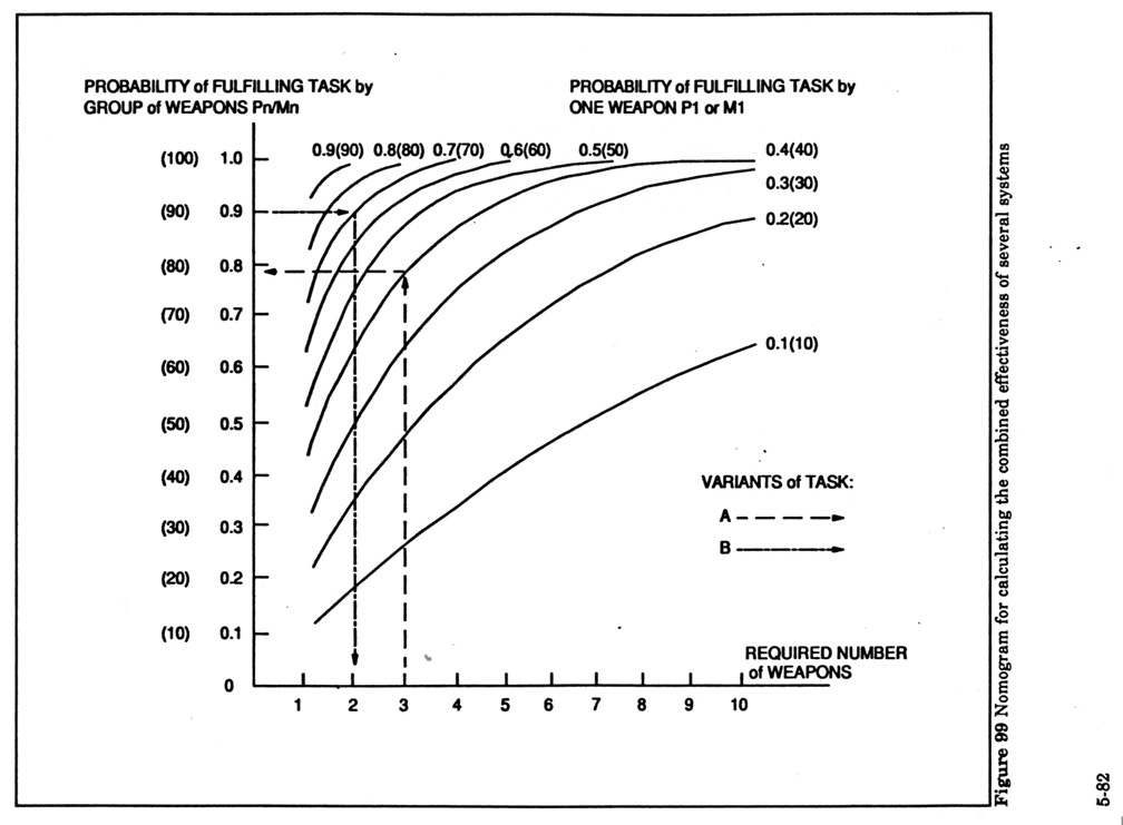
The formula for calculating the effectiveness of different systems fulfilling a
common mission is :
 where Pn is the overall effectiveness of
systems used or in other words the likelihood of fulfilling the mission, and
the individual "P"'s are the effectiveness measures of each system
being summed for the task.
Example: Determine probability of spotting an enemy target with combined use of
3 reconnaissance systems, if their effectiveness expressed as the probability
of detection of enemy target is:
P1=0.4; P2=0.6; and P3=0.8
Solution:
Pn=1 - (1 - 0.4) x (1 - 0.6) x (1 - 0.8)=0.95 or approximately 1.
Example calculations using nomogram Figure 96: Determine the probability of
enemy target destruction with a strike against it by three systems when the
probability of target destruction by a single system of the particular type is
0.4.
Solution: (variant a) Draw a perpendicular from the "3" mark on the
"Required number of systems" scale to the intersection with the
"Probability of mission fulfillment by one system - 4" curve. From
this point draw a horizontal line and on the "Probability of mission
fulfillment by a group of systems" scale read that the probability of
target destruction by three systems is 0.78.
It is possible to determine the reliability of communications in a link which
consists of two channels (n=2), when the reliability of each channel is 0.6.
From the nomogram, the probability of faultless operation of communications in
this instance will be 0.84.
It is possible to evaluate the effectiveness of using four similar
reconnaissance systems to detect an enemy target in an assigned region when the
probability of detection by one system is 0.5. According to the nomogram, the
probability of target detection by four systems will be close to one ).94.
Determine how many weapons systems must be assigned to inflict no less than 90%
damage an enemy target, when the average damage inflicted byu a single system
is 70%.
Solution: Draw a horizontal line from the "0.9" mark on the
"Probability of mission fulfillment by a group of systems" scale to
the intersection with the "Probability of mission fulfillment by a single
system - 0.7" curve. From the intersection point drop a perpendicular line
and on the "Required number of systems" scale find the result - 2.
This means two systems must be used to achieve the assigned damage.
It is possible to determine the required number of communication channels to
provide for 90% reliability when the reliability of a single channel is 0.6.
From the nomogram it appears that at least three channels are required to
ensure this reliability.
From these examples it is evident that the technique may be used for
calculating a wide range of direct and inverse problems associated with the use
of various forces and means. With proper additional factors this method may
also be used to calculate rapidly the effectiveness and required number of
forces and systems when taking into account also probable enemy
countermeasures.
The formulas for calculating the effectiveness of forces and means with
consideration for probable enemy countermeasures are:
 where:
Pn=the probability of mission fulfillment by a group of systems;
P1=the probability of mission fulfillment by a single system of this
type;
Q=the probability indicator of the enemy countermeasure ;
n=the number of forces and means of the given type;
Mn=the mathematical expectation of the damage inflicted by a single
system of this type'
Example calculation: To determine the probability of mission fulfillment by
five weapons systems when the probability of target destruction by a single
system is 60%, while the probability of successful enemy countermeasures is
50%.
Solution: Pn=1 - (1 - 0.6 x 0.5)5=1 - (1 -
0.3)5=0.83.
|
|
| |
Figure 99 Nomogram to calculate combined
effectiveness of several system
|
|
| |
(18) Modeling battle(1)
There is much discussion in the Soviet literature about the theory of
development of coefficients of comensurability. The coefficient is designed to
make it possible to aggregate the effective contribution of various weapons to
a combined arms battle into a composite score for each side. This makes the
measurement of the correlation of forces relatively simple, ie. only one number
for each side rather than the long list of individual types of weapons found in
the standard tables of correlation of forces. However, what sounds simple in
theory is quite difficult in practice. Soviet authors point out that even
within types of weapons such as tanks or artillery the "proving ground
scores" assigned on the basis of technical/tactical characteristics may
not be true reflections of the actual value of the weapon to the commander in
all the diverse conditions of real combat. When it comes to establishing a
uniform score that will place tanks, artillery, aircraft, and small arms, etc
on one scale; a lot of judgment is involved. There is some argument for two
different methods, one would develop a "average" score for each
weapon reflecting its varied value in different circumstances, and the other
method would establish a single theoretical value number and then provide
situation modifiers to be applied to account for each actual set of combat
conditions. We do not have available an actual set of Soviet "utils"
as they call their weapons scores. The following table is taken from a Soviet
article, but the scores are purely hypothetical for educational purposes.
Nevertheless, the following method represents a typical Soviet approach which
may be used by American officers with an appropriate set of "utils".
|
|
| |
Figure 100 Table for coefficients of
comensurability
COEFFICIENTS OF
COMENSURABILITY
|
| Nationality |
Type of combat equipment |
Coefficient of comensurability |
| Country A |
Tank 5 |
1.0 |
| Tank 6 |
1.12 |
| Tank 7 |
1.5 |
| APC |
1.6 |
| AT gun |
0.3 |
| Country B |
Tank 60 |
1.02 |
| APC |
1.4 |
| PTRK |
0.95 |
| AT gun |
0.3 |
| Country V |
Tank 1 |
1.09 |
| APC |
0.45 |
| PTRK |
0.78 |
| RPG |
0.12 |
|
|
| |
Figure 101 Table for expected
loss in combat effectiveness
EXPECTED LOSS IN COMBAT
EFFECTIVENESS
|
| Nationality of forces |
Defense |
Offense |
Meeting battle |
| Prepared |
Non-prepared |
On prepared line |
On unprepared line |
| Country B |
55 |
45 |
30 |
35 |
40 |
| Country V |
60 |
50 |
35 |
40 |
45 |
|
|
| |
The mathematical expectation of the level of
destruction of a side from fire and strikes of artillery and aviation (M) in
the experience of the Great Fatherland War could reach on defense to 40-60% and
on the offense to 20-30%. The losses of combat effectiveness due to destruction
in various types of combat is shown in the table of expected losses. Another
Soviet source gives 30% loss as the critical break point for attackers and 40%
loss as the typical break point for defenders. Of course the effect of losses
on unit combat effectiveness depends heavily on the rate of loss and the size
of the unit.
One more indicator is the coefficient of superiority (Kp) of the
defenders over the attackers, which in the experience of combat typically is
three times.
The possibility of sub-units for destruction of the enemy during the course of
accomplishing their combat missions is calculated according to the following
formulas:
a) in offense:
 b) in defense:
 where:
Ks1, Ks2, Ksp=coefficients of comensurability
of combat means of units of country A;
Kb1, Kb2, Kbp=coefficients of comensurability
of combat means of units of country B or V;
i=quantity of combat means of given type;
Z1, Z2=level of destruction at which the unit loses
combat effectiveness;
M=mathematical expectation of the level of destruction due to artillery and
aviation fire;
Kp=coefficient of superiority of defender over attacker;
S=combat capability of the sub-unit.
For calculations of combat capability during meeting engagement (battle) use
formula (1) but for the coefficient of superiority of defender over attacker
use 1.
Example calculation: The tactical situation; a tank platoon of country A (with
tanks 7) with motor rifle section in a APC has the mission of attacking from
the march to destroy defending section of country B.
Initial data for the calculation:
a. type of combat action is attack;
b. model of combat means of the sides, their quantity and coefficient of
comensurability calculated qualitative indices, are shown in table of
comensurability.
The attackers:
----- tanks "7" Ks1=1.5, and quantity, i=3;
----- APC, Ks2=0.8, and quantity, i=1.
Defenders:
----- APC, Kb1=1.4, and quantity i=1;
----- AT gun, Kb2=0.3, and quantity i=3;
c. the mathematical expectation of the level of destruction of the defenders in
the time of artillery preparatory fire and attack support fire is M=0.4;
d. losses of the sub-unit during the time of approach to the line of going over
to the attack must not exceed Z1=0.3;
e. level of destruction of the defenders at which they loose combat
effectiveness is found in the table of expected loss of effectiveness, Table 2,
Z2=0.55;
Taking the initial data and using formula 1 to create a mathematical model of
the battle gives the following:
-----Sn={[(1.5 x 3) + (0.8 x 1)] x [1 - (0.3 + 0.55 - 0.4)]} ÷
{3 [(1.4 x 1) + (0.3 x 3)] x (1 - 0.4)=0.7
Analysis: If Sn is greater than or equal to 1, then the sub-unit
will fulfill its mission, if (as in this example) the Sn is less
than 1, then the defender with his forces will be superior. This means that it
is necessary to raise the capability if the force to achieve likelihood of
accomplishing the mission.
Decision: Reenforce by fire the platoon on the march from a range of 2000
meters to destroy the enemy APC, and after that conduct fire on the AT gun.
The problem may be decided by means of mathematical modeling of battle:
-----Sn1={[(1.5 x 3) + (0.8 x 1)] x (0.3 + 0.55 - 0.4)} ÷ (3 x
1.4 x (1 - 0.4))=1.19;
In other words, the APC will be destroyed.
-----Sn2={(1.5 x 3 + 0.8 x 1) x (1 - (0.3 + 0.55 - 0.4)} ÷ {3 x
0.3 x 3 x (1 - 0.4)}=1.9.
Outcome: Attacking from the march with forces of three tanks and APC to destroy
an APC and then a AT gun. The line of going over to the attack is designated in
accordance with the characteristics of the terrain, but not closer than 2000
meters from the forward edge of the enemy defenses.
As is evident from the example, the conduct of the calculation is difficult
work demanding a significant amount of time and corresponding conditions. If
the commander has an electronic calculator he could work out the answer
quickly.
What is not evident is to what level of aggregation this method and these
formulas may be taken without loosing validity. The given example illustrates
duels and very small unit combat. With the use of computers it would be
possible to calculate combat at the level of a full regiment or even division
but so many other factors enter in and effect combat outcomes at that level
that a simple formula is no longer valid.
|
|
| |
(19) Calculation of Strike Capability
of Sub-units(2)
This method is designed to calculate the expected depth of penetration of a
unit on the offensive as a measure of its strike capability, or, in reverse, to
forecast the ability of a unit of given combat capability to achieve the depth
of penetration required in its mission. The initial data for the calculation
includes the composition of the attacking and defending units, the conditions
of combat and combat potentials with calculated losses of the sides and also
the designated critical level of losses necessary to cause unit failure.
The critical figure is considered to be the loss at which the sub-unit losses
its combat capability and cannot continue the kind of action it was performing
without re-enforcement. The calculation is made over the width of the front of
the attacker and the designated area of the defense. See the section on
modeling battle for more discussion of the theory and use of the critical level
of loss as an indicator in forecasting and modeling combat. Together these
formulas may be used to determine the initial data on the three measures of
effectiveness described in Chapter One as those deemed critical for assessing
and forecasting battle outcomes.
The formula for calculating the expected depth of penetration follows:

when:
YN (1 - PN ) > (1 - PNK) and
Yo (1 - Po) > PoK)
where:
NN, No=number of units of attackers and defenders,
measured in combat potentials ("utils");
PN, Po=expected losses of the units of each side up to
the arrival at the immediate mission line;
PNK, PoK=critical loss of a unit of
attacker and defender;
FN=width of front of attack in km;
Fo, Go=width of front and depth of the defender's area in
km.
YN, Yo=composition of the units of each side as a
percentage of unity 100%.
K=coefficient of combat effectiveness of the defending side. (This is the same
as Kp in the formulas for modeling battle.
Sample calculation: Determine the expected depth of penetration of attacking
unit whose combat potential at 100% measures 150, during an attack on a enemy
having a combat potential of 194 and a manning of 85%, if the attackers losses
in the immediate battle reach 10% and the defender's losses reach 40%. The
critical loss for the attacker is 50% and for the defender is 70%. The attack
is conducted on a front of 5 km. The defending unit occupies an area of 8 km
wide and 10 km deep, and the coefficient of effectiveness of the defender is
2.5.
Solution:

This means the attacking unit can be expected to succeed in reaching a
depth of 9.5 km in the defender's position. The Soviet author does not indicate
the scale of this combat, and in fact uses the term for sub-unit (ie. a
battalion or smaller), but from the dimensions of the combat area (8 km by 10
km) we may assume this is a regiment attacking of a brigade frontage to the
full depth.
If we use the same formula to evaluate battle at division level we may assume
"utils" of NH=800 for attacker and NO=700 for
defender and the following other values for variables:
YN=90%; YO=80%; PN=0.1%; PO=0.4%;
K=1.5;
PNK=0.5%; POK=0.7%;
FO=20km; GO=30km; FN=15km;
The resulting equation is as follows:
 With these assumptions the attackers may be
expected to achieve a depth of penetration of 53 km.
Using the same formula to evaluate battalion scale combat we may assume both
sides have "utils" of 40, the defender has a superiority coefficient
of 2.5 and the widths are 4, 2, and 1.5 km. Then the formula yields the result
as a penetration of 3.2 km. These are not unreasonable depths for the types of
units being considered.
|
|
| |
(20) Calculation of the Width of Main
Attack Sector
There are several different ways to determine the possible, desired, or
required width of the main attack sector depending on the purposes and
criteria. The following is one quick way to calculate the relationship between
the width of a strike sector and the total width of zone in relation to the
correlation of forces in the strike sector and the total correlation. For these
calculations the correlation of forces may be calculated in terms of
"utils" or in terms of some other aggregate measure based on the
quantities of forces and means of the two sides. The following formula applies:
 where:
Wm=width of strike sector;
Wo=total width of zone;
Co=overall correlation of forces;
Cm=correlation of forces in strike sector;
Cs=minimum desired correlation of forces in rest of zone excluding
strike sector.
Example calculation: Given the width of full zone of action is 120 km, the
overall correlation of forces is 1:1, the correlation of forces in the strike
sector is to be 3:1, and the minimum allowable correlation of forces in the
rest of the area is 0.5:1; determine the possible width of the strike sector.
Solution: Wm=120 (1 - 0.5) ÷ (3 - 0.5)=24 km.
Example calculation: Determine the correlation of forces possible in the strike
sector given that the total width of zone is 400 km, the overall correlation of
forces is 0.8:1, width of strike sector is desired to be 120 km, and the
minimum correlation of forces allowable in the rest of the area is 0.5:1.
Solution: The formula may be restated as Cm=Wo ÷
Wm (Co - Cs) + Cs ; inserting the
given data produces a result of 1.5 as the possible correlation of forces for
the strike sector. The commander may then decide on several alternatives such
as narrow the strike sector, weaken the non-strike sector even more, bring in
reinforcements, or weaken the defenders with preliminary artillery and air
bombardments. Having done the initial calculation the commander may use the
same formula in various ways while deciding on alternatives. For instance, to
determine the required reenforcement to obtain a desired higher correlation the
relationship is C=(1.25 - 0.8) ÷ 0.8 x 100=56.25%, that is by reinforcing
by 56% the correlation in the overall area may be raised from 0.8 to 1.25 to 1.
|
|
| |
(21) Calculation of Required
Destruction of Enemy
Another calculation related to the preceding is to determine what damage should
be inflicted on the defender prior to the attack in order to bring the
correlation of forces into the desired range, considering that there will be a
given amount of loss on the friendly side as well. The formula is as follows:
 where:
M=required level of destruction of enemy in percent;
CN=beginning correlation of forces;
CT=required correlation of forces;
P=forecast friendly losses from enemy action in percent.
Example calculation: In the break through sector regrouping of forces may bring
the correlation of forces to 2:1, however for successful break through we need
to bring the correlation up to 4:1 by means of initial artillery and air
bombardment inflicting losses on the defenders. Determine what level of damage
must be inflicted, if it is expected that the enemy will also inflict 30% loss
on the attacking strike grouping.
Solution: M=100 - 2 ÷ 4 (100 - 30)=65%. Assume that the initial
"utils" of the attackers are 2000 and the defenders are 1000 for a
correlation of 2:1. The enemy will inflict 30% losses bringing the attacking
force to 1400 while the attackers must inflict 65% losses to bring the defender
to 350 "utils" to achieve the 1400/350=4:1 ratio. For more rapid
calculation of this relationship to determine the required losses to inflict
one may use the following nomogram (Figure ). The nomogram is based on the
above formula. The example shown is for the same situation. Enter with the
correlation of forces 2 on the bottom left and draw vertical line to the
correlation of forces 4 line, then a horizontal line across to the 30% loss
line and again vertical down to read the required enemy loss of 65%.
|
|
| |
Figure 102 Nomogram to deermine required
enemy loss to achieve favorable correlation of forces

|
|
| |
(22) Calculation of Rate of Advance
in Relation to Correlation of Forces(3)
Various Soviet articles have discussed the concept of the relation of advance
rates to the correlation of forces of the sides. The relationship is complex
and also depends on several other variables. Evaluation and analysis of the
actual correlations of forces achieved in various operations of World War II
and recent local wars shows that a single norm for the correlation of forces
and means does not exist, but it all depends on the concrete conditions.
Nevertheless sufficient figures to make approximate calculations can be
developed, especially for academic and training purposes. The actual rate of
advance, V, in km per day may be related to a coefficient reflecting the
influence of the correlation of forces, KC, in an equation such as
V=140 x KC. In this the number 140 represents the collected
resulting effect of variables acting in the area, for instance the Western TVD
to give a practical maximum technically possible speed of movement for
mechanized forces in km per day and also an indicator characterized by the
influence of terrain, engineer obstacles, time of year, length of daylight,
etc. The factor KCis a coefficient depending on the correlation of
forces of the sides. This approximate relationship can be shown in a graph.
Analogous graphs can be made for other theaters and conditions. The formula
together with the graph is used to evaluate the formation and determine the
correlation of forces required to achieve a required rate of advance or in
reverse the expected rate of advance for a given correlation of forces.
Example calculation: A given strike group has a planned average rate of advance
of 40 km per day. Determine what the required correlation of forces superiority
is to achieve this rate.
Solution: Taking the formula V ÷ 140=KC or 40 ÷ 140=0.29.
Enter 0.29 on the scale for KC in the nomogram and draw a horizontal
line to the curve and then a vertical line down to the scale of correlation of
forces scale. This shows a required correlation of about 3.4:1 for the strike
sector.
Example calculation: In the zone of action of the strike group we have created
a 2.5:1 superiority in correlation of forces. Determine the approximate tempo
of advance.
Solution: From the nomogram read that the correlation of 2.5:1 corresponds to a
K factor of 0.13. Then using the formula V=140 x 0.13=18.2 km per day advance
rate.
Another approach is to use the following formula to calculate a factor
corresponding to the K factor in the previous method. In the following nomogram
the rate of advance is related also to movement distance, terrain type, length
of the operation and a theoretical maximum movement speed. These variables are
joined into a single factor according to the equation:
F=D ÷ KTVmax
where:
-----D=distance (depth) of operation;
-----K=terrain coefficient (1.25 - level; 1.00 - rough-level; .75 - rugged
hills; .75 - urban; .50 - mtns.)
-----T=time required for operation in days and fractions of days;
-----Vmax=theoretical speed in km per day.
According to this nomogram, to achieve a depth of advance of 30 km on level
terrain in one day with a theoretical maximum speed of 60 km per day requires a
superiority in correlation of forces of 4:1. With a correlation of forces of
3:1 on rough-level terrain and a theoretical maximum speed of 50 km per day in
two days the force may advance 20 km.
|
|
| |
Figure 103 Nomogram that relates correlation
of force to advance rate (1)
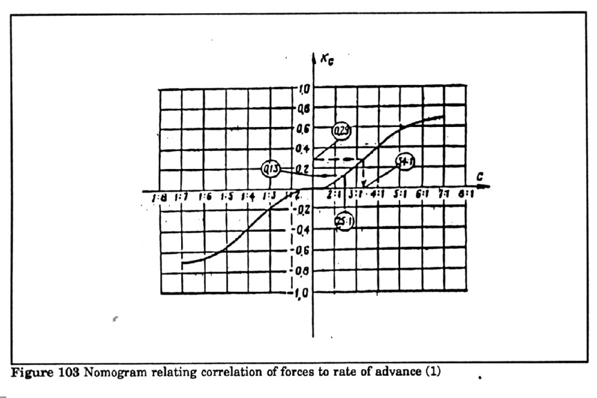
Figure 104 Nomogram relating correlation of forces and rate of advance (2)
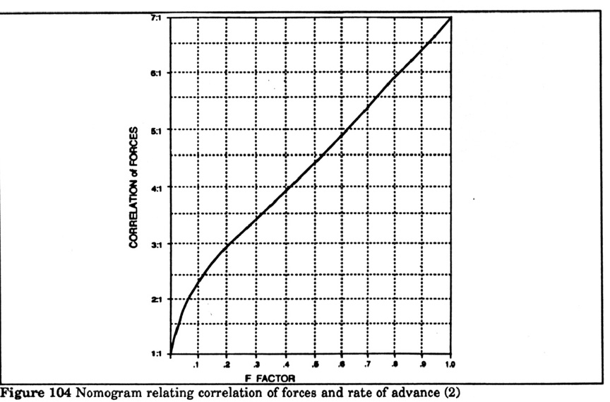
|
|
| |
(23) Determine the Possible Friendly
and Enemy Losses in Relation to the Correlation of Forces and Rate of
Advance
A simplified expression of the relationship between attrition and the
correlation of forces may be shown with a nomogram. In actuality many factors
influence this relation, however, for general planning at frontlevel
the averages shown in the nomogram may be sufficient. This nomogram is built
with the following assumptions.
1. The attacker needs a 3:1 advantage represented by the line at 45 degrees to
break even and have the same loss rate as the defender.
2. The losses to each side are related to the force ratio in a relatively
simple and direct way, but the greater the force ratio advantage and the longer
the time interval the larger the difference in attrition will be. So losses
accumulate faster for the side with the disadvantage in forces;
3. For an army size force the losses are about .5% per day when the correlation
of forces in 1:1
|
|
| |
Figure 104 Nomogram for
calculation of force attrition Army
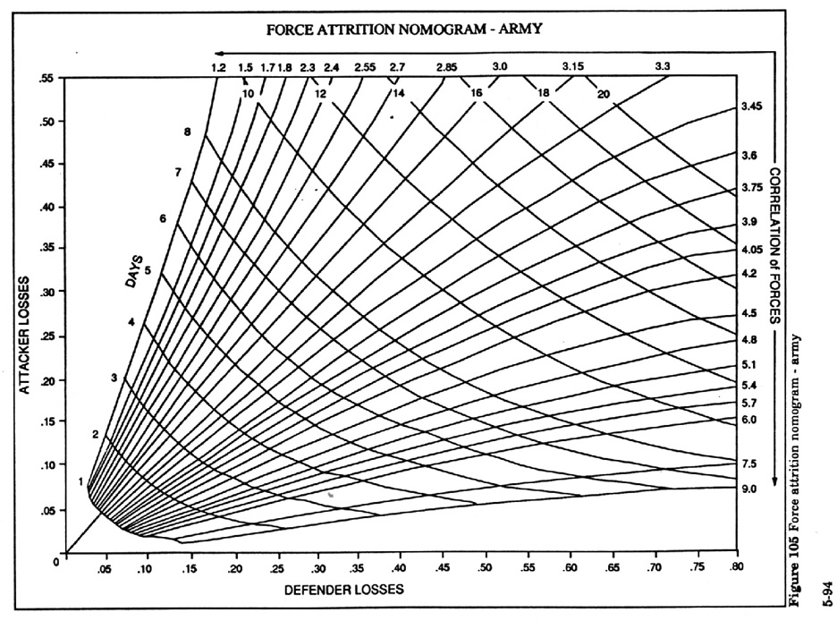 |
|
| |
Figure 106 nomogram for calculation of
attrition - front
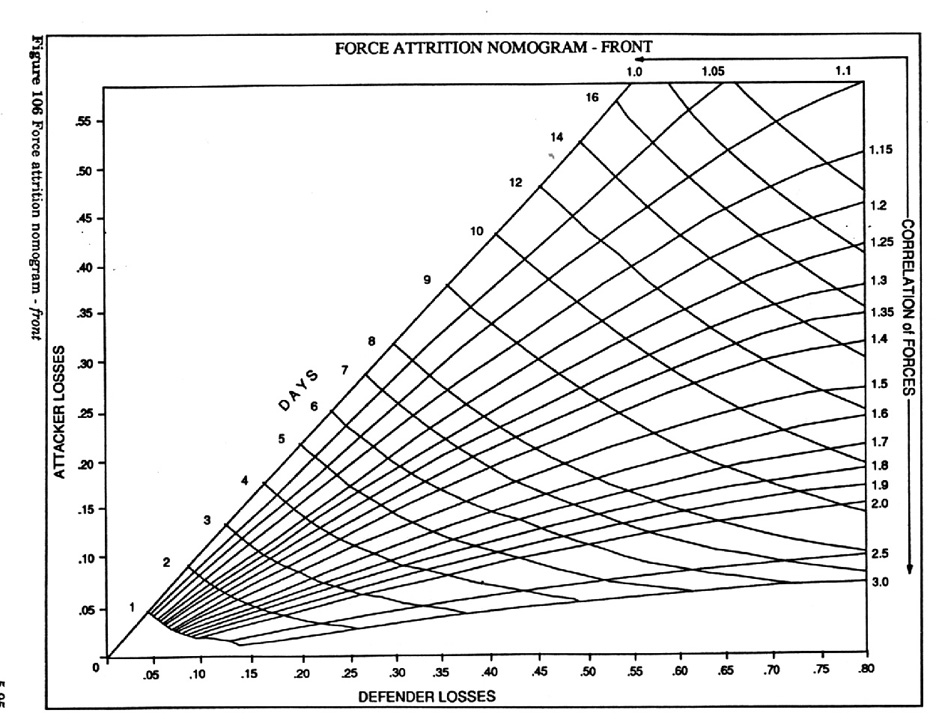
|
|
| |
(24) Determine the Required Amount of
Manpower and Weapons for Bringing Sub-Units back up to Sufficient Strength to
Restore their Combat Capability
This calculation is made to determine how many men and weapons are needed to
restore the sub-unit or unit to combat capability sufficient to accomplish the
mission. It is not expected that the replacements will restore the sub-unit to
its original full strength, but just to the necessary ratio of correlation of
forces and means between the two sides. The mission was determined in the first
place on the basis of a calculated correlation of forces and means deemed
sufficient (such as 3:1). Since both sides have suffered losses the quantity
required to restore the original favorable correlation will not equal the loss.
The basic data needed for the calculation are information on the original full
strength of the troops of the two sides, the losses sustained and the
superiority ratio of correlation of forces and means required for carrying out
the task. The results of the calculation represent the quantities necessary to
restore the force to its combat capability. Combat capability in this case
means sufficient strength to accomplish the mission. Obviously this is one of
the most important calculations Soviet commanders must make during combat. The
formulas for the calculation are:
Mi=Ci - Ai ÷ Bi ;
Ai=(nf Pf) x Nf ;
Bi=(ne -Ne Pe) x Ne ;
mi=Bi x Mi
where.
M=index of the reduction of combat capability in terms of the required ratio of
manpower and weapons for the execution of the mission;
Ci=required degree of superiority ratio for a particular type of the
i type of weapon;
Ai=availability remaining on hand quantity of weapons of a
particular type i of own forces;
Bi=availability of remaining number of weapons of a particular type
i for enemy forces;
nf (ne)=initial full strength of own troops (enemy
troops) by type i of weapons pers/ proportions;
Pf (Pe )=losses of own troops (enemy troops)
pers/proportions;
Nf (Ne )=TOE number of weapons of a particular type i of
own forces (enemy forces);
mi=number of weapons of a particular type which are required for the
restoration of own troops combat capability.
If M is less than 0 then the calculation is no longer performed since the
filling out of the forces and means is not required to restore combat
capability. This method may be used both in calculating the number of various
types of combat equipment, as well as in calculating the correlated
quantity/quality indicators.
What these formulas mean essentially is that M is an index showing the reduced
combat capability of friendly forces in terms of the change in the correlation
of forces resulting from the differential losses by the two sides. It is equal
to C (the required correlation of forces ) minus the actual ratio (correlation)
of forces.
The term "A" is the remaining quantity of forces or means of the
particular type for friendly forces and it is equal to the initial strength
minus the product of the friendly initial strength times the losses to friendly
forces all times the TOE strength.
The term "B" is the same thing for the enemy forces.
Then m is the quantity of the forces or means required to restore the initial
favorable (required) correlation and it is equal to the remaining strength of
the enemy (B) times the M index of reduced combat capability (deficit in
correlation)
Example calculation using the table: Determine the required number of tanks and
guns to re-equip a sub-unit if the required level of superiority is 2.5:1, the
initial full strength of own troops was 85% (0.85), the losses of own forces in
tanks is 40% (0.4), the initial full strength of the enemy was 60% (0.6), his
losses in tanks are 40% (0.4).
Solution: Entering the data in the table we find that to resupply the sub-unit
and restore its combat capability requires 2 tanks. Replacements of guns are
not required since, given the losses on both sides, the required level of
superiority necessary to fulfill the mission is preserved.
|
|
| |
Figure 107 Form for the Calculation
of the Required Amount of Personnel
CALCULATION OF FORCES AND MEANS TO
RESTORE COMBAT EFFECTIVENESS
|
| No |
Initial data, values and operations to be
determined |
Unit
(Accuracy)
|
Forces and equipment |
| Tanks |
Guns |
Mortars |
BTR |
Etc |
| 1 |
Initial full strength of friendly forces |
percent |
0.85 |
0.7 |
|
|
|
| 2 |
Friendly forces losses |
percent |
0.4 |
0.2 |
|
|
|
| 3 |
Tabular volume of friendly force equipment |
units |
25 |
32 |
|
|
|
| 4 |
(1) x (2) |
(0.01) |
0.34 |
0.14 |
|
|
|
| 5 |
(1) - (4) |
(0.01) |
0.51 |
0.56 |
|
|
|
| 6 |
(3) x (5) |
(1.0) |
13 |
18 |
|
|
|
| 7 |
Initial full strength of enemy forces |
percent |
0.6 |
0.6 |
|
|
|
| 8 |
Enemy forces losses |
percent |
0.4 |
0.3 |
|
|
|
| 9 |
Tabular number of enemy force equipment |
units |
18 |
25 |
|
|
|
| 10 |
(7) x (8) |
(0.01) |
0.24 |
0.18 |
|
|
|
| 11 |
(7) - (10) |
(0.01) |
0.36 |
0.42 |
|
|
|
| 12 |
(9) x (11) |
(1.0) |
6 |
10 |
|
|
|
| 13 |
Established degree of superiority of friendly forces (proceeding
from the ratio of forces and equip) |
|
2.5 |
1.5 |
|
|
|
| 14 |
(6) ÷ (12) |
(0.01) |
2.17 |
1.8 |
|
|
|
| 15 |
(13) - (14)* |
(0.01) |
0.33 |
-0.3 |
|
|
|
| 16 |
Number of equipment required to fill out: (12)
x (15)
|
units (1.0) |
2 |
- |
|
|
|
| * At (15) is less than 0, there is no need
to fill out the forces and equipment, the subunit is combat ready and may
successfully fulfill the established mission. |
|
|
| |
(25) Determine the Expected Radiation
Dose
The initial data for this calculation are the length of travel route within the
zone of radioactive contamination, the average radiation level on the travel
route and the speed and direction of travel of the sub-units. The degree of
shielding of the personnel is assigned by a coefficient of radiation reduction
by the transport equipment. The formula is:
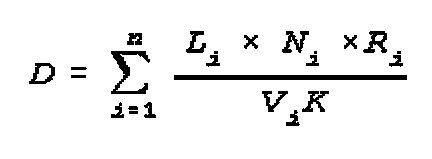
where:
D=the expected radiation dose of personnel in roentgens;
Li=the length of the route within the i zone of radioactive
contamination in km;
Ni=factor which considers the direction of zone relative to the axis
of the radioactive pattern. (If travel is along the axis of the pattern N
equals 1, and if perpendicular to the axis N equals 0.25, and at an angle to
the axis N equals 0.375);
Ri=mean radiation level on the travel route in roentgens per hour;
Vi=the speed of travel in km per hr;
K=the coefficient of reduction of radiation by the protection of the transport
equipment;
n=the number of zones to be crossed.
Example calculation using the form: Determine the possible radiation doses of
personnel of a subunit while they are negotiating two zones of radioactive
contamination with mean radiation levels of 187 and 165 roentgens per hour. The
length of the route within the first zone is 12 km and the second is 10 km. The
travel speed of the sub-unit is 25 and 18 km per hr respectively. The first
zone is crossed along a route perpendicular to the pattern axis and the second
at an angle to the pattern axis. The reduction coefficient is 4.
Solution: performing the calculations using the table we find that the total
radiation dose received by personnel may reach 15 roentgens.
The formula and method for calculation may be simplified by considering the
entire zone as a whole and using average values for the above variables. In
this case the expected dose of radiation may be expressed as D=(R x L) ÷
(K x V);
and the required speed of movement is V=(R x L) ÷ (K x D);
This relationship is shown on the following nomogram.
Example calculations using the formulas: Determine the anticipated dose of
radiation of personnel crossing a sector of radio-active contamination with a
level of 78 R/hr, if the length of route is 18 km, the sub-unit speed is 25
km/hr, and the coefficient of protection is 7. The solution is 8 roentgens.
Determine what is the required speed to negotiate a contaminated zone 17 km
deep when the mean radiation level is 95 R/hr, the protection coefficient is 4
and the allowable radiation level for personnel is less than 20 R. Solution is
approximately 20 km/hr.
Example calculations using the nomogram: Determine the expected personnel
radiation dose from passing through a sector of radio-active contamination of
60 R/hr, when the length of route is 12 km, the unit travel speed is 15 km/hr
and the protection coefficient is 2. Solution: (Variant A) From the
"12" mark on the "Length of sector of contaminated route"
scale draw a perpendicular line to the intersection with the "Average
level of radiation - 60" line. From that point draw a horizontal line
through the obtained point to the intersection with the "Speed of movement
15" line and then draw a vertical line to the "Coefficient of
degradation 2" line." From that point draw a horizontal line to the
"Dose of radiation of personnel scale, on which read the result=24
roentgens.
(Variant B) is to calculate the speed for negotiating a contaminated zone so
that the personnel will receive less than 48 roentgens when the route length is
18 km, the radiation level is 80 R/hr, and the coefficient for protection is 2.
Draw a perpendicular line from the 18 mark on the "Length of sector"
line to intersect with the "Average level of radiation - 80" line and
draw a horizontal line to the left. Then draw a horizontal line from the
"48" mark on the "Dose of radiation of personnel" line to
the intersection with the "Coefficient of degradation - 2" line and
from that point draw a vertical line to intersect with the previously drawn
horizontal line. The intersection point on the "Speed of Movement"
lines at the 15 line shows that 15 km/hr is the minimum acceptable speed for
crossing the contamination.
Another method for calculating the expected radiation dose for personnel may be
used with a nomogram by considering only averages over the entire width of the
radiation zone. The initial data for this calculation are the length of the
contaminated section of the route, the mean radiation level over the route, the
unit travel speed during passage of the contaminated area, the degree of
shielding of personnel by the vehicles. This method is used to calculate the
speed required to pass the contaminated area so that personnel do not receive a
larger radiation dose than allowed. The formulas are: D=RL ÷ KV; and V=RL
÷ DK
where:
D=the expected radiation dose of personnel in roentgens;
L=the length of the route in km;
R=mean radiation level on the travel route in roentgens per hour;
V=the speed of travel in km per hr;
K=the coefficient of reduction of radiation by the protection of the transport
equipment;
The mean radiation level is determined on the basis of radiation reconnaissance
data by averaging the readings at various points along the route.
Example calculations using the formula: Determine the expected radiation dose
for personnel in crossing a radioactive zone 18 km deep when the mean radiation
level is 78 roentgens per hr, the sub-unit travel speed is 25 km/hr, and the
reduction coefficient is 7.
The solution is D=78 x 18 ÷ 7 x 25=8 roentgens.
To determine the speed required to cross a contaminated area 17 km deep when
the mean radiation level is 95 roentgens/hr, the reduction coefficient is 4,
and the allowable radiation level is less than 20 roentgens. The solution is:
V=95 x 17 ÷ 4 x 20=20 km per hr.
Example calculations using the nomogram Figure 105: Variant A: Determine the
expected personnel radiation dose in crossing a contaminated zone with
radiation level of 60 Roentgens/hr when the length of route is 12 km, the
travel speed is 15km/hr and the reduction coefficient is 2.
Solution: From the 112 mark on the "contaminated route length" scale
draw a perpendicular line to the intersection with the "Mean radiation
level - 60" line. From this point draw a horizontal line to the
intersection with the "Travel speed - 15" line. Draw a vertical line
through this point to the intersection with the "Reduction coefficient -
2" line and then draw a horizontal line to the "Personnel radiation
dose" scale. At that point read the result=24 roentgens.
Variant B: Determine the speed for crossing a contaminated zone so that the
personnel receive less than 48 roentgens, when the route length is 18 km, the
mean radiation level is 80 roentgens per hr, and the radiation reduction
coefficient is 2.
Solution: Draw a perpendicular line from the 18 mark on the "contaminated
route length" scale to the intersection with the "Mean radiation
level - 80" line and then draw a horizontal line to the left. Draw a
horizontal line from the 48 mark on the "Personnel radiation dose"
scale to the intersection with the "Reduction coefficient - 2" line
and through this point draw a vertical line to the intersection with the
previously draw horizontal line. The point of their intersection on the
"Travel speed - 15" line shows the result is 15 km/hr. This is the
minimum speed required.
|
|
| |
Figure 108 Form for calculating expected
radiation doses
FORM FOR CALCULATING EXPECTED RADIATION DOSES
|
| No |
Initial data, calculations to be
performed |
Units and accuracy |
Calculation variant |
| Example |
2 |
3 |
| 1 |
Length of route within the first zone of radioactive
contamination |
km (1.0) |
12 |
|
|
| 2 |
Travel speed |
km/hr (1.0) |
25 |
|
|
| 3 |
Factor for travel direction |
(0.001) |
0.25 |
|
|
| 4 |
Average radiation level |
R/hr (1.0) |
187 |
|
|
| 5 |
Radiation reduction factor for transport
equipment |
(0.1) |
4 |
|
|
| 6 |
(1) ÷ (2) |
(0.01) |
0.48 |
|
|
| 7 |
(6) x (3) |
(0.01) |
0.12 |
|
|
| 8 |
(7) x (4) |
(1.0) |
22 |
|
|
| 9 |
Radiation dose of personnel: (8) ÷
(5) |
R (1.0) |
6 |
|
|
| 10 |
Route length in second radiation zone |
km (1.0) |
10 |
|
|
| 11 |
Travel speed |
km/hr (1.0) |
18 |
|
|
| 12 |
Factor for travel direction |
(0.01) |
0.375 |
|
|
| 13 |
Average radiation level |
R (1.0) |
165 |
|
|
| 14 |
Radiation reduction factor for transport
equipment |
(0.1) |
4 |
|
|
| 15 |
(10) ÷ (11) |
(0.01) |
0.56 |
|
|
| 16 |
(15) x (12) |
(0.01) |
0.56 |
|
|
| 17 |
(16) x (13) |
(1.0) |
35 |
|
|
| 18 |
Personnel radiation dose: (17) ÷
(14) |
R (1.0) |
9 |
|
|
| 19 |
Total dose: (9) + (18) |
R (1.0) |
15 |
|
|
|
|
| |
Figure 109 Nomogram to calculate expected
radiation doses
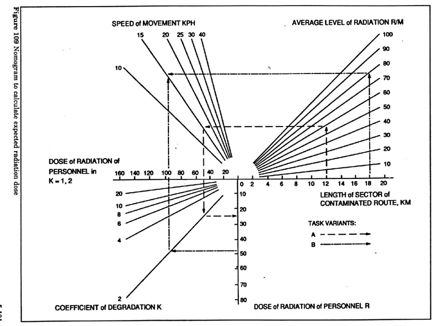
|
|
| |
(26) Calculation to Select the
Optimal Travel Route
This is an extremely important and varied class of calculation. The example
given here is only illustrative of the possibilities for employing the given
method for solving problems of optimization from among a small set of possible
variants.
The commander of a sub-unit has a mission to break out to an assigned line and
assume the defense in the shortest possible time. There are five possible
travel routes to reach the assigned position. All routes pass through a zone of
radioactive contamination. Therefore, an additional condition of the advance is
the expected dose of radiation received by sub-unit personnel. It is apparent
that in this example there are five decision variants. The main criterion for
evaluating their relative effectiveness is the travel time. The shorter the
better. However, the commander must also strive to keep the received radiation
dose at a minimum, or at least not allow it to exceed a set maximum per norms,
for instance 50 roentgens.
The conditions for the sub-unit to advance to the assigned mission line may be
expressed in a table showing quantitative characteristics. From the data it
becomes obvious that the possible movement routes differ from each other in
length, road quality, and mean level of radiation.
From the table we see that on route 1 in advance variant 1 there are four
segments of 16 km of highway, (travel speed 40 km/hr) 10 km of improved dirt
road (travel speed 25 km/hr), 9 km of dirt road (travel speed of 15 km/hr), and
5 km of damaged, nearly impassable road (travel speed < 5 km/hr). The mean
radiation level on the entire first route is 100 roentgens per hr. From this
information we can calculate the expected duration of travel time to reach the
mission line, as follows:
-----t1=(16 ÷ 40) + (10 ÷ 25) + (9 ÷ 15) + (5 ÷
5)=2.4 hrs or 2 hrs, 24 min. The first route passes through a radiation zone of
100 roentgens per hr. Using the previous method for calculating radiation with
a reduction factor of K=4 for equipment D=(100) (2.4) ÷ 4=60 roentgens.
After calculating the same data for the other four routes the information
needed for the decision may be shown in another table of movement time and
expected radiation dose.
|
|
| |
Figure 110 Table to enter description of
travel routes
QUANTITATIVE CHARACTERISTICS OF ALTERNATE ROUTES
|
| Advance route number |
Length, km, of route segments of different
road quality |
Mean radiation level on route,
R/hr |
| 1st |
2nd |
3rd |
4th |
| 1 |
16 |
10 |
9 |
5 |
100 |
| 2 |
-- |
20 |
12 |
4 |
120 |
| 3 |
29 |
12 |
6 |
2 |
120 |
| 4 |
-- |
15 |
20 |
5 |
60 |
| 5 |
16 |
15 |
3 |
4 |
80 |
| Travel speed along each segment km/hr |
40 |
25 |
15 |
5 |
|
|
|
| |
Figure 112 Table of effectiveness of
alternate routes
|
|
| |
EFFECTIVENESS
INDICATORS FOR TRAVEL ON VARIOUS ROUTES
|
| Route (variant) number |
Time to move forward (hr) |
Expected radiation dose, R |
| 1 |
2.4 |
60 |
| 2 |
2.4 |
72 |
| 3 |
2 |
60 |
| 4 |
3 |
45 |
| 5 |
2 |
40 |
|
|
| |
These results may now be compared to
determine the optimum decision of which route to choose. Displaying this data
in the table makes it easy to see that the optimum solution is route number 5,
having both the shortest travel time and lowest radiation dosage, however this
might not always be the case. We can also see that the shortest route (no 2) is
actually worse than the longest ( no 3). However, a more general technique for
solution, when the answer is not evident is to prepare a graph to plot the
information. In this example plot the radiation dose on the y axis and the
travel time on the x axis. Then enter the coordinates for the given mission
requirements, such as maximum travel time of 3 hrs and maximum radiation dose
of 50 roentgens. Draw vertical and horizontal lines from the axes to the
selected coordinates. Plot the data for all the possible variants. Those
variants whose position falls within the rectangle formed by the axes and the
lines to the decision point.
|
|
| |
(27) Calculation to Determine Optimal
Distribution of Weapons
One of the most important classes od decision for the commander is the optimal
distribution of weapons against various targets. This is a more complex
calculation that the previous example of optimum route given two decision
criteria. As an example consider the distribution of weapons against a group of
targets. The calculation technique shows the course and result of the
calculation for optimization. Of course, the ideal solution technique is to use
computers, and Soviet headquarters are certainly using this method. In the
field, however, the commander may be required to make a rough calculation
without having a computer available. The following simple method produces
sufficiently reliable results when a small number of forces and means and
targets are being considered. The illustration, nevertheless, indicates the
type of problem for which computer solutions may be developed.
In this example the commander must find the most effective distribution of five
different groups of weapons against five strong points in order to inflict the
maximum casualties on the enemy. having calculated the effectiveness of fire of
each of the groups of weapons against each target, for instance, using the
technique with the nomogram ( ) the commander may create a table of
effectiveness of damage to each enemy target by each weapon.
|
|
| |
Figure 113 Table of effectiveness of
artillery fire on targets
EFFECTIVENESS OF
ARTILLERY FIRE DAMAGE ON TARGETS
|
| Weapons group |
Damage effectiveness in
hectares for target number |
| 1 |
2 |
3 |
4 |
5 |
| 1 |
3 |
4 |
3 |
5 |
9 |
| 2 |
4 |
7 |
5 |
4 |
7 |
| 3 |
6 |
8 |
3 |
5 |
9 |
| 4 |
2 |
6 |
9 |
8 |
5 |
| 5 |
9 |
4 |
2 |
2 |
4 |
|
|
| |
The damage achieved by different weapons
against various types of targets is not identical because of the difference in
the quantity and quality of the weapons, the quality of the shells, and the
relationship of the ballistic characteristics of the weapons (dispersion
pattern etc) to the dimensions of the targets, and the degree of shelter of the
enemy personnel.
According to the data in the table, the first group of weapons when hitting the
first enemy target inflicts casualties to the personnel in an area of 8
hectares, the second weapons group against the same target damages 4 hectares,
and so on.
If the commander assigns the first weapons group against the first target, the
second group to the second target, etc., then the effectiveness of the
distribution will be the total area damaged or 30 hectares. However, this
solution will not be optimal, since the actual combat capabilities of the
available weapons in these conditions are not used in the best way. In order to
find the best distribution and solve the problem quickly, another method for
calculation must be used. The initial data for this are shown in the next
table; the weapons groups, the number of target groups and the firing
effectiveness.
The calculation of the optimal distribution is performed directly on the table.
First, select the two greatest values for the effectiveness values in each
line. In the first line these are 9 and 8, and in the second they are 7 and 7,
etc. Then subtract the lesser value from the greater and write the results in
the right hand column, as shown. Perform the calculation first by each line and
then by each column. Examine the differences by lines and columns, select the
greatest value and mark it (*). In this example the result is the fifth line,
but the maximum may also be in a column. Then in the line or column in the
fields for which the greatest value shows, find the maximum indicator and
underline it. (This is the 9 in line 5 column 1.) This indicates that the fifth
weapons group should be targeted against the first target group. Eliminate this
pair from further consideration.
The course of the further calculation is shown in the next table. The remaining
weapons are in a similar manner distributed against the remaining target groups
until all groups of weapons are distributed.. This shows that the first group
should fire on the fourth target, the second on the second, the third against
the fifth, and the fourth against the third. This results in the greatest
damage to enemy personnel, a total area of 42 hectares. This is the maximum
value of damage from the 120 possible combinations of weapons and targets in
the example.
|
|
| |
Figure 114 table of effectiveness of
artillery fire on targets
EFFECTIVENESS OF
ARTILLERY FIRE DAMAGE ON TARGETS (COURSE I)
|
Course 1 |
| Weapons group |
Damage effectiveness in
hectares for target number |
| 1 |
2 |
3 |
4 |
5 |
| 1 |
8 |
4 |
3 |
5 |
9 |
1 (9-8) |
| 2 |
4 |
7 |
5 |
4 |
7 |
0 (7-7) |
| 3 |
6 |
8 |
3 |
5 |
9 |
1 (9-8) |
| 4 |
2 |
6 |
9 |
8 |
5 |
1 (9-8) |
| 5 |
9 |
4 |
2 |
2 |
4 |
5* (9-4) |
| C-1 |
1 (9-8) |
1 (8-7( |
4 (9-5) |
0 (8-8) |
0 (9-9) |
|
|
|
| |
Figure 115 Table of effectiveness of
artillery fire on targets
EFFECTIVENESS OF
ARTILLERY FIRE DAMAGE ON TARGETS (COURSE I)
|
Course 1 |
C 2 |
C 3 |
C 4 |
| Weapons group |
Damage effectiveness in
hectares for target number |
| 1 |
2 |
3 |
4 |
5 |
| 1 |
8 |
4 |
3 |
5 |
9 |
1 (9-8) |
1 |
1 |
- |
| 2 |
4 |
7 |
5 |
4 |
7 |
0 (7-7) |
0 |
0 |
0 |
| 3 |
6 |
8 |
3 |
5 |
9 |
1 (9-8) |
1 |
1 |
1 |
| 4 |
2 |
6 |
9 |
8 |
5 |
1 (9-8) |
1 |
- |
- |
| 5 |
9 |
4 |
2 |
2 |
4 |
5* (9-4) |
- |
- |
- |
| C-1 |
1 (9-8) |
1 (8-7( |
4 (9-5) |
0 (8-8) |
0 (9-9) |
|
|
|
|
| C-2 |
- |
1 |
4* |
0 |
0 |
|
|
|
| C-3 |
- |
1 |
- |
3* |
0 |
|
| C-4 |
- |
1 |
- |
- |
2* |
|
|
|
| |
In this example the total area of damage was
considered the indicator of effectiveness. Sometimes one must minimize the
effectiveness indicator instead of maximizing it. For instance, the indicator
might be the time required for fulfilling the mission, the expenditure of
munitions or other materials, etc. Top optimize the distribution according to a
minimum indicator value, use the same technique, only in calculating the
differences in the lines and columns, select two minimum values instead of the
two maximum ones and subtract the least from the greatest. Then find the
minimum indicator in the appropriate line or column and fix it first.
This comparatively simple and practical technique for determining the optimum
distribution of forces and means is useable in the field. The materials being
distributed might be weapons, reconnaissance means, communications systems,
water crossing equipment, etc.
|
|
| |
(29) Calculation to Determine the
Effectiveness of Fire Destruction Means
This is a more elaborate version of the basic formula designed for use with
calculators. The initial data is the number of fire targets, the number of
weapons, rate of fire, and coefficient of effectiveness of fire, the length of
time for conducting fire, and the coefficient of resistance (counteraction) of
the enemy.
Formula is:
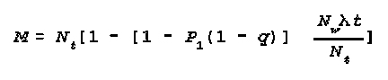
where:
M=quantity of targets to be destroyed;
Nt=total number of targets;
Pi=probability of destruction of target from one weapon by one shot;
q=probability of destruction of weapon by fire of enemy;
Nw=number of weapons;
=rate of fire (number of rounds per min);
t=duration of fire in min.
Example problem: Determine the expected number of destroyed targets from 30
observed targets, if 12 weapons with a rate of fire of 3 rounds a minute are
used for their destruction. The probability of destruction by 1 shot is 0.2 and
firing time is 5 min. The probability of destruction of our weapon by enemy in
the time of one shot is .3
|
|
| |
Figure 116 Form for calculating weapons
effectiveness
FORM FOR CALCULATING WEAPONS EFFECTIVENESS CONSIDERING ENEMY
COUNTERMEASURES
|
| No |
Initial data and values to be
determined |
Units |
Calculation variant |
Remarks |
| Example |
2 |
3 |
| 1 |
Number of targets |
units |
30 |
|
|
|
| 2 |
Probability of destruction in one shot |
-- |
0.2 |
|
|
|
| 3 |
Probability of destruction by enemy during one shot |
-- |
0.3 |
|
|
|
| 4 |
Number of weapons |
units |
12 |
|
|
|
| 5 |
Firing rate |
rounds / min |
3 |
|
|
|
| 6 |
Firing time |
min |
5 |
|
|
|
| 7 |
Number of destroyed targets |
units |
18 |
|
|
|
|
|
| |
Reconnaissance Planning
Reconnaissance planning makes use of many of the same calculations and formulas
used for operational planning, such as time and distance for movements and
optimization of resources. The following are some calculations specifically
designed for reconnaissance planning.
|
|
| |
(30) Calculation of Effectiveness of
Reconnaissance and Required Duration for a Reconnaissance Mission
The given data for the calculation is the speed of movement of the
reconnaissance means, the actual range of observation of reconnaissance, the
dimensions of the area being covered and the duration of the patrol
The formula is:
 where:
P=probability of observing an object (target);
e=natural logarithm 2.72;
R=radius of observation of targets by reconnaissance in km;
V=rate of movement of reconnaissance means during the mission in km/hr;
t=duration of patrol;
S=area of the region being observed in sq km.
If it is required to observe several targets in one area, then the mathematical
expectation of coverage (average number of targets seen) for observed targets
can be calculated as M=N x P
where M=average number of observed targets; N=total number of targets in the
area;
and R=probability of detection of one target.
To determine the duration of patrol in order to observe a target with a
pre-determined likelihood for observation the formula is:
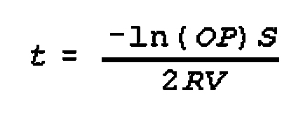 |
|
| |
Example problem: Determine the likelihood of
observation of targets after 2 hours of reconnaissance in an area of 58 sq km
if the effective observation distance is 1.5 km and rate of movement of the
patrol is 12 kph. The table shows the answer that the probability of
observation coefficient is .71. Answer is that if there are 15 targets in the
area then they can find 10 to 11 of them.
|
|
| |
Figure 117 Form for calculating probability
of target detection
Figure 117 Form for calculating probability of target detection
FORM FOR CALCULATING
PROBABILITY OF DETECTING TARGETS
|
| No |
Initial data and values to be
determined |
Units |
Calculation variant |
Remarks |
| Example |
2 |
3 |
| 1 |
Effective target detection range |
km |
1.5 |
|
|
|
| 2 |
Reconnaissance system speed |
km/hr |
12 |
|
|
|
| 3 |
Search duration |
hr |
2 |
|
|
|
| 4 |
Search region area |
sq km |
56 |
|
|
|
| 5 |
Target detection probability |
-- |
0.71 |
|
|
|
|
|
| |
Example problem 2: Determine the duration of
time to perform the reconnaissance mission to observe a target in an area of 50
sq km to a likelihood percentage of 80%, if observation distance is 1.2 km and
rate of movement is 15 kph.
Answer is 4.5 hr
|
|
| |
Figure 118 Form for
calculating search length
FORM FOR CALCULATING LENGTH OF RECONNAISSANCE SEARCH
|
| No |
Initial data and values to be
determined |
Units |
Calculation
variant |
Remarks |
| Example |
2 |
3 |
| 1 |
Target detection probability |
-- |
0.8 |
|
|
|
| 2 |
Search region area |
sq km |
50 |
|
|
|
| 3 |
Effective target detection range |
km |
1.2 |
|
|
|
| 4 |
Reconnaissance system speed |
km/hr |
15 |
|
|
|
| 5 |
Search duration |
hr |
4.47 |
|
|
|
|
|
| |
(31) Calculation of Detection of
Targets by Reconnaissance
If the probability of detection of targets at a given range may be considered
as approaching 1, then the formula for calculating the probability of detecting
a target in an area during a patrol of given length can be simplified to
eliminate the logarithm. The simplified formula may in turn be structured into
a nomogram for even faster calculations. In this case the initial data for the
calculation are the length and speed of the search, and the range of reliable
target detection ( probability near 1.0) of the reconnaissance systems. The
formula is:
 where:
2RVt is less than or equal to S;
P=probability of target detection;
R=effective range of reliable observation in km;
V=search speed in km per hr;
t=search time in hours;
S=surface area of the search region in square km.
Example calculation using formula: Determine the probability of target
detection in 2.5 hours in an area of 37 sq km when the search speed is 4 km/hr.
Solution is P={2 x 1.3 x 4 x 2.5} ÷ 37=0.7
Example calculation using the nomogram Figure 112: Determine the probability of
detection of a target in 3 hrs in an area of 50 sq km, when the range of
detection is 1.2 km and the search speed is 6 km/hr.
Solution: For this calculation (variant a) draw a perpendicular line from the
"1.200" mark on the "Reliable detection range" scale to the
intersection with the "Search speed - 6" line. From the point draw a
horizontal line to the right to intersect the "Search length - 3"
line, then from this point draw a horizontal line to the left to the
"Probability of detection" scale. Read the answer at 0.86.
Example 2: Determine the search length in an area of 60 sq km, when the target
detection probability is 0.9, the reliable detection range is 1.3 km and the
search speed is 8 km/hr.
Solution: For this calculation (variant b) draw a horizontal line to the right
from the "0.9" mark on the "Probability of detection" scale
to the intersection with the "Search region area - 60" line. From
this point draw a vertical line. Then draw a perpendicular line from the
"1.300" mark on the "Reliable detection range" scale to the
intersection with the "Search speed - 8" line. From this point draw a
horizontal line to the right to the intersection with the previously draw
vertical line. They intersect along the "Search length - 2.5" line.
The answer then is approximately 2.5 hours required to complete the assigned
search.
|
|
| |
Figure 119 Nomogram to calculate probability
for target detection

|
|
| |
Sample Calculations for Division and
Army Staff
Example calculation using formulas: On the basis of army's initial instruction
the division staff calculates the time its lead regiment requires to move to
the border area and deploy there when:
----- depth of regiment column - 30 km
----- depth of the area of deployment - 6 km
----- average speed of march - 20 km
----- distance to the border area - 120 km
|
|
| |
Solution:
Use the formula:
 where:
t=time the regiment needs to deploy in new area
D=distance to border area
V=average speed of march
GK=depth of regiment column
GR=depth of the area of deployment
tp=time spent for halts
t=(120 ÷ 20) + (30 - 6) ÷ (0.6 x 20) + 1=9 hrs
Example calculation: On the basis of the same instructions the division
determines the time for the division to deploy and occupy the designated
departure area when:
----- depth of division columns on 3 routes - 80 km
----- depth of the area of deployment - 35 km
----- average speed of march - 25 km
----- distance to departure area from start line - 125 km
----- time to complete engineer work - 8 hours
Solution: To solve the problem the staff applies a combination
of calculations and norms. Calculations are done both in general terms (time to
complete the deployment for the entire division) and calculations to determine
the time of deployment of different echelons such as first and second echelons,
rear service troops, air defense troops, attack helicopters etc. The method is
the same for all categories. In each case normatives are applied to determine
the time required for specific tasks such as engineer work, establishment of
fire system, delivery of supplies, loading and unloading, establishment of
security, etc.
A. Calculations in general terms:
T=(D ÷ V) + tp + (Gk - GR) ÷ 0.6V +
tengr
T=125 ÷ 25 + 1 hr + (80 - 35) ÷ (0.06 x 25) + 8 hrs
T=5 + 1 + 3 + 8=17 hrs.
B. Calculations in specific terms
1. For the first echelon regiments (depth of column 30 km, depth of area of
deployment 10 km):
 where:
T=(150 ÷ 25) + 1 + (30 - 10) ÷ (0.6 x 25) + 8 hrs ....(1)
T=6 + 1=1:20 + 8 hrs=16:20 hrs
2. For second echelon regiments use the same formula:
T=170 ÷ 25 + 1 + (30 - 10) ÷ (0.6 x 25) + 8 .....(2)
T=6:48 + 1 + 1:20 + 8=17.08
3. For the rear service use the same formula:
T=195 ÷ 25 + 1 + (10 - 5) ÷ (0.6 x 25) + 8 ......(3)
T=7:48 + 1 + 0.20 + 8=17:08
Notes:
(1) Movement distance for first echelon regiments is assured to be 150 km on
the basis that the regiments should move another 25 km from the division
deployment line to reach there designated position in the first echelon (125 +
25=150)
(2) The distance for the second echelon is assumed to be 170 km on the basis
that the regiment moves 35 km from the head of the column (depth of first
echelon regiment plus 5 km interval) and to reach its designated area it should
move another 10 km from the divisions to reach its area of deployment in the
second echelon (125 + 35 + 10=170 km)
(3) The distance for the rear service is assumed to be 195 km to include its
distance from the head of the column (65 km) and the 5 km interval (125 + 65 +
5=195 km)
Example problem: The division commander must clarify his
mission and calculate the following on the basis of the army commander's
instructions.
----- depth and width of the division missions;
----- width of the area of penetration;
----- required rate of advance;
----- number of regiments required in first and second echelon.
Solution:
1. The depth and width of the division mission is measured on the map in
the following manner:
----- depth of the immediate mission 17 km with a width of 8 km
----- depth of long range mission is 21 km and a width of 12 km
----- the width of penetration area is 3.5 km, requiring the forces and means
of two regiments (2 km and 1.5 km of penetration area assigned to them), the
remaining 4.5 km of the front should be covered by part of one of the regiments
of the penetration area (the right flank regiment) and forces and means of
another regiments.
2. The immediate mission to be accomplished in ------- hours (assume 7 hours)
therefore the average rate of advance is 17 ÷ 7=2.5 km/h. The long range
mission is to be accomplished in ------ hours (assume 5 hours), therefore the
average rate of advance should be 21 ÷ 5=4 km/h
3. On the basis of the width of penetration area which is 3.5 km (the norm is 2
km per regiment) and the overall width of the division sector i.e. 8 km there
can be two alternatives for the echelonment of the troops:
a. Two regiments in the first echelon, one BMP regiment covering the
front and one regiment in the second echelon to be committed after the
penetration of the enemy's brigade defensive position, while the BMP regiment
will then constitute the second echelon to be committed after the penetration
of enemy's division defenses.
b. Three regiments in first echelon, with the BMP regiment coming to the second
echelon after the attack is begun.
4. Therefore the commander can tentatively determine the following:
----- rate of advance
----- direction of the main attack and the width of penetration area
----- combat formation of the division for the attack
5. Issues mentioned in point 4 are further examined , elaborated and confirmed
during the estimate of the situation and "recognasirovka".
Example problem: As the chief of operation section prepare for
the commander calculations to determine the required correlation of forces and
means to support the assigned rate of advance.
Solution: To solve the problem use the rate of advance
nomogram. To use the nomogram first find the F factor
----- F factor=D ÷ KTVmax;
----- D=distance (depth) of the mission
----- K=terrain coefficient:
----- 1.25 level
----- 1.00 rough-level
----- .75 rugged hills
----- .75 urban sprawl
----- .50 mountainous
----- T=time required for action in days and fraction of days
----- Vmax=theoretical speed in km/day
-----F=38 ÷ (1.25 x 1 x 60)=0.5
Now see in the nomogram what correlation of forces and means is required when
the F factor is 0.5 The answer is 4.3:1
Example problem: Determine the width of the main sector on the
basis of the following facts:
----- width of the overall area of the division is 8 km
----- overall correlation of forces and means is 3: 1
----- required correlation of forces in the main sector is 4.3:1
----- correlation of forces and means below which we can not drop in the rest
of the division area is 2:1
Solution: Use the size of the sectors formula which is as
follows:
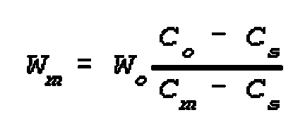
where:
Wm=width of the main sector
Wo=width of the overall area
Co=overall correlation of force
Cm=required correlation of force
Cs=correlation of force below which one can not drop in the rest of
the action area.
Wm=8 (3 - 2) ÷ (4.3 - 2)=3.5 km
Note:
You can increase the width of the main sector area by accepting a lower
correlation of forces and means in the rest of the area of division attack, for
example:
Wm =8 (3 - 1.3) ÷ (4.3 - 1.3=13.6 ÷ 3=4.5 km
Example problem: Calculate the time for a division to advance
from the assembly area (departure area) and deploy for shift into attack from
the line of march when:
----- distance of attack line from enemy forward line=1 km:
----- distance of line to deploy into company column=4 km:
----- distance of line to deploy into battalion column=12 km:
----- distance of regulating line to line of deployment into battalion
column=20 km:
----- distance of regulating line from start line=40 km:
----- distance of start line from assembly area=5 km:
----- depth of first echelon regiments=30 km:
----- interval between 1st and 2nd echelon regiments=10 km:
----- movement speed into attack=8 km:
----- average speed during march=24 km/h:
Solution: This calculation can be done either by using several
formulas to calculate each section of the advance and finally to combine them
together or by filling in prepared tables.
a. Using formulas:


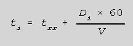

 ta=time for crossing final deployment
into line of attack minus (H) in minutes:
Da=distance of line for going into attack formation from the forward
edge of the enemy position in km:
Va=rate of movement in attack formation in km/h:
tr=time for crossing the line of deployment into company column (H
-minutes):
Dr=distance of line of deployment into company columns from the line
of deployment into attack formation in km:
v=average rate of movement of units in mounted formation during march:
tb=time for crossing line of deployment into battalion column (H
-minutes):
Db=distance of line of deployment into battalion columns from line
of deployment into company columns in km:
trr=time for crossing the last regulation line (LRL) prior to
deployment into battalion columns (BC):
Drr=distance of LRL to BC:
ti=time for passing the start line (SL):
Di=distance of SL from LRL:
tvit=time to begin movement from assembly area
D=distance of SL from assembly area:
ti'=time for crossing the SL by second echelon:
Gk=depth of the mounted column of first echelon in km:
Dk=distance between the tail of the first echelon and the head of
the second echelon in km:
60 and 90=coefficient for conversion of time in minutes for the average speed
during the deployment on each line:
ta=(1 x 60 ÷ 8=7.5 ( H - 7.5 min)
tr=7.5 + (4 x 90) ÷ 24=7.5 + 15 min=(H - 22.5 min)
tb=22.5 + (12 x 60 ÷ 24=22.5 + 30 min=(H - 53 min)
trr=52.5 + (20 x 60) ÷ 24=52.5 + 50=(H - 1hr,43 min)
ti=01:43 + (40 x 60) ÷ 24=01:43 + 01:40=(H - 03:23)
tvit=03:23 + (5 x 90) ÷ 24=03:23 + 00:19=(H - 03:42)
ti'=03:42 + (30 + 10) x 90 ÷ 24=03:42 + 02:30=(H -
06:12
b. Using the tables:
The same calculations can be done by using the tables given above with the
individual calculations and filling in the numbers in each line. Such tables
are pre-prepared in advance in blanks and the operation staff can use them to
do calculations taking different options into consideration.
Sample calculations: Determine the time and distance to the line of meeting
with a counter-attacking enemy reserve when:
----- the enemy reserve (up to 2 mech and 2 tank battalions) is sighted 28 km
from the forward line of division's attacking troops:
----- enemy's speed of advance is about 15 km/hr:
----- a delay of 30 minutes is expected in the enemy movement due to a narrow
area along the road:
----- planned air strikes and artillery fire's are expected to delay the enemy
for another 40 minutes:
----- the speed of own attacking forces in the first echelon is 4 km/hr due to
isolated enemy's strong points across the front:
----- the attack on enemy's position 4 km further in the depth (the troops are
expected to reach there within an hour) is expected to delay 45 minutes for
minor regroupment.
Solution:
Use the following formula:
 where:
tv=expected time of meeting the enemy in hours:
D=distance between opposing forces in km
tn=total delay time for own forces in hours
Vn=speed of movement of own forces
tp=total delay time for enemy forces
Vp=speed of movement of enemy forces
Results:
tv={28 + [(0.75 x 4) + (1.15 x 15)]} ÷ (4 + 15)
tv=[28 + (3 + 17.35)} ÷ 19
tv=(28 + 20.25) ÷ 19 : tv=2.54 or 2 hrs and 33
minutes
Now to determine the distance of meeting with the enemy use this formula:
lp=Vn (tv - tn )
lp=4 (2.54 - 0.75)
lp=7.16 km
This means that the first echelon forces will be able to destroy the enemy in
this intermediate defensive position before it can launch its counter-attack,
provided the enemy's reserve is delayed by air strikes and artillery fire for
not less than 40 minutes and the enemy does have to slow down 30 minutes delay
to cross the narrow pass and own forces do not take more than 45 minutes to
regroup in order to continue the attack.
If the division commander determines that the line of meeting with the enemy is
not convenient, he can chose to repel the counter-attack from a line further in
back or he might want to further delay the enemy so that the first echelon
troops can move further than 7.16 km before the enemy launches his
counter-attack. This calculation can also be conducted by filling in the
pre-prepared form.
Example calculation: On the basis of the assumptions which were mentioned in
exercise 10 determine the number of anti-tank weapons (ATGM and AT guns) to
repel the enemy tanks when:
----- the number of enemy tanks are estimated to be 80:
----- no less than 50% of enemy tanks must be destroyed:
----- the probability of destruction of a single tank by one weapon with one
shot is 0.2:
----- up to 8 rounds may be fired by each weapon in the time the tanks are
located in the effective zone of fire:
Solution: To determine the required number of anti-tank
weapons use the formulas or the nomogram.
Formulas;

 where:
Mn=degree of destruction of tanks by artillery (in percentage);
P1=probability of destruction by one weapon in one shot;
N=required number of anti-tank weapons to accomplish the mission;
m=weapon rate of fire or number of shots one weapon can shoot during the time
the target is in within range;
M=expected number of attacking tanks.
This method is a lengthy one and difficult to use under field conditions.
The nomogram can be used for up to 40 tanks. However, for over 40 tanks divide
the number into pieces less than 40 and calculate on the basis of the nomogram
and add the results: 60=40 + 20, or 77=40 + 37 etc.
In this example the following calculation can be done on the nomogram: Draw a
perpendicular line from 0.5 mark on the "Required amount of destruction of
targets" scale to intersect with the "Probability of target
destruction by one round 0.2" curve. From this point draw a horizontal
line to the intersection with the "Number of attacking ground targets -
40" line and then a vertical line up to the "Number of firing by one
weapon - 8" line. From this point go along the horizontal to
"Required number of antitank weapons" scale and read 17 then multiply
it by 2 to get the required number of AT weapons for 80 tanks: 17 x 2=34 AT
weapons.
Example calculation: The division commander decided to use the divisional AT
reserve at the line for repulsing the enemy's counter-attack, which previous
exercise set at 7 km up from the current forward line of the first echelon
troops. The AT reserve is now 8 km from the forward line. The enemy is 21 km
away from the line of repulsion of counter-attack with an expected delay of 1
hour and 10 minutes on the way (due to planned air strikes and artillery's
fire). The speed of advance of the enemy is 15 km/hr the effective range of AT
weapons is 3 km. The AT reserve will need 30 minutes to deploy on the fire line
and prepare for action. It's speed of movement 12 km/hr.
Determine how much time is available for the division commander and staff to
assign mission to the AT reserve.
Solution:
Use the following formula:
 where:
t=time available for the commander and his staff to assign mission;
D=distance of the enemy to the line of contact;
tp=total delay time for enemy forces;
Vp=speed of movement of enemy forces;
d=effective range of AT weapons;
tn=total time required for AT reserve to move to the line of the
repulsion of the enemy's counter-attack and time to prepare for action.
1. First determine the tn:
 where:
tn=time for AT reserve to move and prepare for action;
Vn=speed of movement of AT reserve;
tr=time to prepare for action;
tn=(8 + 7) ÷ 12 + 0.5=1.75.
2. Now determine the t:
t={[D + (tp x Vp)] - d} ÷ Vp -
tn
t={[21 + (1.15 x 15)] 2} ÷ 15 - 1.75
t=[(21 + 17.5) - 2] ÷ 15 - 1.75
t=(38 - 2) ÷ 15 - 1.75
t=36 ÷ 15 - 1.75
t=2.25 - 1.75=0.5
t=30 minutes.
This means that the division commander and staff should assign mission to the
AT reserve within 30 minutes (not later) so that the AT reserve will arrive and
get prepared on the line of repulsion before the enemy tanks reach the
effective range of AT weapons at the line.
Example calculation: In planning the commitment of divisions's second echelon
the area within 4 km of the enemy intermediate defensive position, which is to
be attacked by the second-echelon, is open and when the regiment moves and
deploys to company and platoon columns and assumes the combat formation in this
area, it should be covered by artillery strikes conducted on enemy strong
points at the line of commitment and on the flanks. The line of attack is 1 km
and the line of fire safety is 400 m from enemy position. The speed of movement
is 20 km/hr and speed of attack is 6 km/hr. Determine the duration of artillery
strike to cover the deployment and attack of the second-echelon regiment.
Solution: To determine the duration of artillery strike
calculate the time it takes the regiment to deploy and move to the line of
attack and then to the safety line of fire in front of enemy position (400m).
Use equations:
t=ta + tr ...........(1)

 where:
t=time of artillery strike;
ta=time for crossing the attack line up to the fire safety line;
tr=time spent from deployment in the company columns up to the line
of attack;
Da=distance of attack line from enemy position;
d=distance of fire safety line to the enemy position;
Va=speed of movement in attack;
Dr=distance of deployment into company columns;
V=speed of movement of troops;
Results:
ta=(1 -0.4) x 60 ÷ 6=6 minutes
tr=3 x 90 ÷ 20=27 ÷ 2=13.5 minutes
t=ta + tr=6 + 13.5 approximately 20 minutes
This means that the artillery strike should be conducted for 20 minutes to
cover the commitment of the second echelon regiment.
Example calculation: The division has accomplished its immediate mission and
continues the attack in depth to complete the destruction of the enemy forces
in its tactical zone and accomplish the long range mission by the end of the
day. The first echelon regiments are fighting with the enemy forces, which
conduct delaying action and cover the withdrawal of its main forces across the
Schmalin River. Two enemy battalion size columns 15 km from the river are
withdrawing to the river apparently to establish defense on the river. The
division commander has decided to assign a forward detachment to prevent the
arrival of these enemy battalions on the river. The distance to the enemy
columns from the head of the assigned forward detachment is 15 km. A 20 minute
delay is expected in the movement of enemy columns due to planned friendly air
strikes. The speed of movement of enemy's columns is 15km/hr.
Determine the expected time and rate of overtaking of the withdrawing enemy by
division's forward detachment.
Solution: Here the crucial issue is to overtake the enemy
before he is able to cross and establish defense at the river.
1. First determine how long does it take the enemy to reach the river:
t=D + (tp x Vp) ÷ Vp
t=time it takes the enemy to reach the river;
D=distance of the enemy to the river;
tp=expected delay in enemy's movement;
Vp=speed of enemy's movement;
Results:
t=[15 + (0.5 x 15)] ÷ 15
t=(15 + 7.5) ÷ 15=22.5 ÷ 15=1.5
t=1 hr and 30 minutes
Therefore the enemy's columns must be overtaken within less than 1.5 hours.
2. Assume that the speed of movement of the forward detachment is 20 km/hr:
Now to=[D - (tp x Vp )] ÷ (Vn
- Vp )
to=time to overtake the enemy (hours);
D=distance to the enemy;
tp and Vp=same as in 1;
Vn=speed of movement of own forces (forward detachment);
to=15 - (0.5 x 15) ÷ (20 - 15)
to=(15 - 7.5) ÷ 5
to=7.5 ÷ 5=1.5
to=1 hour and 30 minutes
This means that at a speed of 20 km/hr the forward detachment can not catch the
enemy columns before they reach the river. In order to overcome this, either
the speed of movement should be increased or the enemy should be further
delayed by air strikes, airborne assault troop, artillery fires, mines etc.
3. In order to find the required speed of movement of the forward detachment to
overtake the enemy in one hour perform the following calculation, using the
formulas:
Vn={[D - tp x Vp)] + (to x
Vp)} ÷ to
Vn=[15 - (0.5 x 15)] + [(1 x 15)] ÷ 1
Vn=(7.5 + 15) ÷ 1=22.5 ÷ 1=22.5
Vn=22.5 km/hr.
Therefore the speed of movement of the forward detachment should be at least
22.5 km per hour to ensure the enemy's interception within an hour. At that
time the enemy will be 7.5 km from the river.
D=(t x Vp) - (tp x Vp)
D=(1 + 15) - (0.5 x 15)
D=15 - 7.5=7.5 km
Calculations for Front Offensive Planning
One of the most important preliminary calculations made by the
front commander is for the allocation of his forces to first and
second-echelons and to main and secondary attack axes (directions). This is
done on the basis of the correlations of forces required to achieve assigned
results in the attack sectors and the minimum correlations allowable in other
(holding attack) sectors. In addition the quantity of artillery available to
meet density norms will also be a governing factor.
Example calculation: Presume the initial instructions received by the
front commander establish the following: the front is
assigned a mission for offensive operation with the scope:
----- overall depth: 640 km
----- depth of immediate mission: 280 km
----- depth of long range mission: 360 km
----- width of the frontage: 340 km
----- duration of operations 14 days
The front is composed of four combined arms armies on D day, a tank
army will join the front on D + 2. During the clarification of the
mission the commander determines the following:
----- number of attack directions and breakthrough areas;
----- number of armies in the first echelon;
----- rate of advance, and required correlation of forces for such rate of
advance.
Answer:
Since the direction of the main attack is determined by the superior commander,
the front will facilitate the establishment of the appropriate
grouping of forces and means and support of the axis. In this case the
front also has a choice to determine the number of supporting attacks
and forces allocated to them.
1. On the basis of initial data the front has one direction of main
attack. According to theory a major part of the forces should be allocated to
this direction: two armies with a frontage of not more than 60 km in a European
type of terrain (60 x 2=120 km of front). Now what is left is 340 - 120 + 220
km. Therefore this 220 km is to be covered by two more armies.
If the front launches a supporting attack with one army, it cannot
give the army a sector of more than 80 km.
(therefore: 220 - 80=140 km).
Now if one army is assigned this 140 km front, it cannot attack; but only will
hold the line or it may attack in a narrow sector merely to support the main
attack of the supporting attack directions.
These are preliminary deductions based on the clarification of the mission.
These variants can be further developed during the estimate of the situation.
The determination of the number and overall width of the breakthrough areas
depends on the number of armies and divisions in the first echelon. This is
again a tentative and rough assessment, while the more detailed calculation can
be conducted later, on the basis of artillery capability and number and type of
enemy targets.
Penetration areas:
----- main direction: 2 armies each 12 km=24 km
----- supporting direction: 1 army 10 km - 10=total of 34 km
2. Rate of advance:
----- a. 640 ÷ 14=45 km/day
This is the average rate of daily advance which should be maintained. In order
to see if this rate of advance can be maintained, make an overall and summary
correlation of forces and means. A 3:1 correlation supports an average rate of
advance of 40 to 60 km/day.
----- b. To find out the required correlation of forces and means (basically on
the main direction) use the formula/nomogram of ("Correlation of forces
needed for rates of advance") That is Figure 103 above:
----- f (factor)=D ÷ KTVmax;
----- f=correlation factor;
----- k=terrain factor (1.25 for open terrain);
----- Vmax=theoretical speed in km/day.
On the nomogram read that a correlation of 4.6 to 1 is required to achieve the
accomplishment of the mission in 14 days. This is a rough calculation and the
enemy's detailed capabilities are not taken into consideration. This
correlation mostly applies to the axes of main attack, while on axes with
holding attacks a lower correlation can be accepted.
Assume that the four divisions attacking in the right flank army and the three
divisions attacking in the army adjacent to it to the south are the main
direction.
On the supporting direction three divisions of the left flank army attack in
the first-echelon with one division of the adjacent army to the north
participating in the breakthrough. Determine the overall breakthrough area and
number of artillery pieces required.
Answer:
1. Main direction: 4 divisions + 3 divisions=7 divisions: the norm for the
width of the breakthrough area per division is 4 km. Therefore 7 x 4=28 km.
General norm for number of artillery pieces required per km of breakthrough
area is 100 (90-110). Therefore 28 x 100=2800 artillery pieces.
2. Supporting direction: 3 divisions + 1 division=4 divisions: 4 x 4=16 km
(width of breakthrough area): 16 x 100=1600 artillery pieces.
Exercise calculation: Determine the correlation of forces and means in the
holding area when overall correlation of forces and means is 3:1 and as
discussed in the above exercise, the width of the main sector is 120 km, of
supporting attack sector 80 km, and overall width of front'soperation
area is 340 km. The required correlation of forces and means on the main
direction as discussed above is 4.6 to 1 and in the supporting direction is 4
to 1.
Answer: Use the following formula:
 1. Main sector versus the entire front:
120=340 (3 - Cs) ÷ (4.6 - Cs)
552 - 120 Cs=1020 - 340 Cs
220 Cs=468 ÷ 220
Cs=2
Therefore in the rest of the frontage (out of the main sector and overall
correlation of 2:1 is required.
2. Supporting sector versus the rest of the front (340 - 120=220 km)
80=220 (2 - Cs) ÷ (4 - Cs)
320 - 80 Cs=440 - 220 Cs
140 Cs=120; Cs=120 ÷ 140=.85
Cs=.85
It means that if we establish a 4:1 correlation of forces and means in the
supporting attack sector, the overall correlation of forces and means in the
rest of the front (excluding the main and supporting attacking sectors) cannot
be more than 0.8:1 which will support only defensive action.
3. Suppose that the army which will be assigned in this 140 km sector between
the main sector (120 km) and supporting attack sector (80 km) decides to launch
attack by one division in a 20 km sector with a 3:1 correlation to support the
flank of the main or supporting attack sectors. In this case the overall
correlation of forces and means in this sector will further drop from its
original 0.85:1. Here is how it calculates using the same formula above.
20=140 (0.85 - Cs) ÷ (3 - Cs)
60 - 20 Cs=119 - 140 Cs
120 Cs=59; Cs=59 ÷ 120
Cs=0.5
This means that if the army launches a division size attack in part of its
sector (20 km) then the correlation of forces and means in the rest of the
sector will drop to 0.5:1 or the enemy will have a superiority of 2:1 in this
sector. If a temporary defensive action can be acceptable to the front
commander in this sector, then the army can choose this course of action.
|
|
| |
Calculating Operational Scale Rates
of Movement(4)
|
|
| |
The necessity for evaluating terrain
passability in a zone of prospective operations arises equally with the study
and analysis of its protective and maskirovka qualities every time an
offensive operation is planned and conducted or when troops are regrouping or
maneuvering. This is natural since passability of terrain is an important
operational factor for successful troop movements and actions in an
operation.(5)
Passability of terrain in the operational plan depends on the relief features,
the presence of large forests, the density and condition of the road network,
hydrologic and soil conditions as well as on natural obstacles, barriers, and
the amount of destruction in the zone of troop operations. These qualities of
terrain have a significant effect on determining the overall operational plan,
its scale, the selection of main axes of operations, the depth of mission, the
forms and methods of deployment, logistical organization, engineer effort, and
other types of operational support.
It is know that the speed of troop movement and the most efficient organization
of their combat formation depend greatly on the quantity and type of obstacles
on the routes of march. When planning a march or regrouping on an operational
scale calculations are also complicated by the fact that troop movements must
be carried out in a concentrated manner along several parallel routes in
strictly specified periods of time with minimum expenditure of personnel and
equipment for the preparation of march routes and for keeping them in passable
condition. In order to fulfill all these requirements it is necessary to
consider some conditions determining a subsequent operational decision.
The most important of these conditions are as follows:
----- sufficient distance between routes of march to insure the safety of
troops moving on any one of them in case of an enemy nuclear attack on the
adjacent route;
----- the quantity and location of routes of march which are most consistent
with the operational plan;
----- efficient traffic loads on the routes of march to achieve not only
maximum rate of traffic on each of them, but also the highest possible total
rate of traffic on routes of march to insure organized movement within
prescribed periods of time.
In effect this means that the greater traffic carrying capability on the route
of march the more troops should be moved over it. It is important to apply such
a procedure not only when considering the operational plan, but also when
calculating the simultaneous movement of the main body of forces to an assigned
area or to the deployment position.
The most convenient criterion determining traffic carrying capability of a
given route of march is the average speed of movement over it. It takes into
account not only the march speed of the columns, based on the technical
condition of the road and the tactical-technical characteristics of the
equipment involved, but also various delays en route connected with restoring
the route of march or maintaining it in passable condition. Such an approach to
evaluating passability of routes of march takes into account changing
conditions in the conduct of operations when the factor of time and high speeds
of movement become decisive.
The traffic carrying capability of a road is understood as the quantity of
combat or transport vehicles passing over it in a prescribed interval of time.
Traffic carrying capability is determined according to the following formula:
 Where:
N=the number of motor vehicles and other combat vehicles passing through in one
hour;
Sav=the average speed of movement (meters/hours);
ll=the minimum distance between vehicles (meters);
lo=the overall length of the motor vehicle (meters)
This formula reflects the tactical and technical sides of the problem. However,
for operational calculations it cannot be used in this form for two reasons.
First, this concept of traffic carrying capability does not take into account
the peculiarity of troop movement in march formation, when a definite distance
is established between separate columns. Second, according to the computed
value for traffic carrying capability it is difficult to draw the correct
conclusions required for solution of operational problems. Obviously, for
operational calculations it is more expedient to introduce the concept of
operational-tactical traffic carrying capability, which can be determined by
the quantity of formations and units passing through in a prescribed time
period over a given route of march. Operational-tactical traffic carrying
capability of a route of march is determined according to the following
formula:
 where:
P=the operational-tactical traffic carrying capability of a route of march (the
quantity of formations and units passing through in one hour). When calculating
major operational regroupings consideration should be given to specific
features of the column for each branch of troops, for the amount of available
equipment of losses suffered and other data which make possible determination
of approximately equal depth in route order of large units or units for
application during actual conditions.);
Sav=average speed of column movement, km/hr;
K=the number of large units or units moving along the route of march;
De=depth of march formation of troops (km).
As a result the traffic carrying capability as well as the speed of movement
computed according to the given formula can describe the passability of a route
of march in the form of a numerical indicator. When planning a major maneuver
of troops in any particular zone it is important to determine not only the
passability of individual routes of march, but also the overall passability of
terrain in the zone. The characteristic passability of a zone can be its
traffic carrying capability, which will depend on the quantity of routes of
march, the speeds of movement over them by large columns, and on the
organization of the march formation. Traffic carrying capability in a
particular zone (Pz) can be defined as the sum of
operational-tactical traffic carrying capabilities available on its routes of
march (P), i.e.:
Pz=/P (3)
Thus, the criterion for traffic carrying capability of a zone can be taken
as the quantity of large units and units, with a typical length of march
formation for the given conditions, passing through the entire zone in the
given period of time.
For example: In the zone there are four routes of march. On the basis of
operational and tactical requirements and the evaluation of conditions on the
routes of march the average rates of speed were established as follows: on
route 1 -- 25 km/hr; on route 2 -- 19 km/hr; on route 3 -- 28 km/hr and on
route 4 -- 20 km/hr.
On each of them moves a column of troops consisting of five troops consisting
of five troop units with a given composition and an overall depth of march
formation of (De) equaling 200 km. The traffic carrying capacity of
each route is determined according to formula (2) and the following results are
obtained:
-----for route 1 -- P1=25.5 ÷ 200=0.6; for route 2 --
P2=19.5 ÷ 200=0.5;
-----for route 3 -- P3=28.5 ÷ 200=0.7; for route 4 --
P4=20.5 ÷ 200=0.5.
Operational tactical traffic carrying capability for the entire zone is
determined according to formula (3) -- Pz=0.6 + 0.5 + 0.7 + 0.5=2.3.
This means that over the given zone in the period of one hour there can pass
through two troop units with a typical or characteristic depth of march
formation for the determined conditions as provided in the given instance.
The operational/tactical traffic carrying capacity of march routes, as seen
from formula (2), depends on the speed of movement, the overall depth of the
march formation, and the quantity of large units and units traveling over the
route of march.
For this reason it is most important to use all means to increase speed of
movement and decrease the length of the troop column. In addition to careful
reconnaissance of routes of march and engineer support on each route, it is
also expedient to make up a march graph. Such planning increases the
independence of columns during regrouping and will promote increased speed of
troop movement and, consequently, traffic carrying capacity on the routes of
march. Where possible as many troop routes as possible should be designated to
reduce the overall depth of the march formation. It is advisable to assign the
best routes of march to troops forming a substantially long column.
When preparing for an operation or during its progress the quantity of routes
of march for troops will be determined on the basis of the operational
disposition of the troops, available roads in the theater of military
operations, total traffic capacity of the roads, availability of time for
movement and the distance involved, as well as the expected enemy action with
weapons of mass destruction. To take all these factors into consideration and
make a decision quickly on the allocation of the required number of routes of
march for any particular large unit will be, undoubtedly, quite difficult.
After proper analysis and research the mathematical function of those factors
have been determined and expressed by the following formula (4):
 where:
K=the quantity of routes of march;
a=the coefficient determining the relationship between the average speed of
movement, Sav, to the actual speed during forward movement or
deployment, Sfm, of the troop column.
a=Sav ÷ Sfm;
De=depth of the march formation (km) during movement along one route
of march;
T=the time allotted for the movement (hours);
Sav=the average speed of movement (km/hr);
D=the distance on the route of march (km).
Assume that the troops are required to complete a march over a distance where
D=200 km at an average speed of Sav=25 km/hr in a time of T=12 hrs;
the depth of the march formation during movement over only one route of march,
De, is 200 km, and the speed during forward movement
Sfm=12.5 km/hr. According to the given formula it is possible to
calculate how many routes should be prepared or assigned, with the computation
as follows:
[(25 ÷ 12.5) x 200] ÷ [(12 x 25) - 200]=400 ÷ 100=4
For rapid calculations under field conditions it is more convenient to use
graphs or nomograms. In this connection a proposed graphic variant in the form
of a nomogram is provided for determining any particular unknown parameter when
evaluating the passability of terrain over the routes of march.
Shown on the nomogram as an example is the graphic determination of the
quantity of march routes based on the data contained in the above formula. From
the point T=12 hours, located on axis O-T, a perpendicular is drawn to the
intersection of the slant line corresponding to the speed of movement
V=25km/hr. From this point a horizontal line is extended to the left to
intersect with the line where D=200 km. Then a perpendicular is dropped to the
curve when De=2100 km and then a horizontal line is extended to the
right. The required quantity of march routes is indicated on the axis O/K.
The nomogram provided is constructed on the assumption that:
----- a=Sav ÷ Sfm=2.
In this case if the relationship between the speeds of movement of all the
route of march and during deployment between the speeds of movement of all the
route of march and during deployment are different from the prescribed, then
the value of K, determined graphically, of necessity will increase on the
corrected coefficient a1, based on the change in speeds.
In formula (4) and in the nomogram the same speed of movement is used over the
entire route of march. In practice, even in preliminary evaluation of march
routes, the speed can vary. In case the difference in speed of the march does
not increase more than 10-15 percent, then during operational calculations (by
formula or on the Nomogram) the average speed of movement over all selected
routes is used. To assure the simultaneous appearance of troops in the
designated area it is advisable to have the troop columns proportional to the
possible speeds of movement. If the difference in speeds of movement turns out
to be substantial, then initially a determination is made on troop groupings
which can complete the march over the best roads in the allotted period of
time. Mathematically this means that according to formula (4) with a given
value K the depth of the march formation De is determined. After
this the remaining quantity of troops is distributed over the routes of march
which permit slower speeds of movement and calculations are made according to
the same formula.
With the aid of formula (4) and the nomogram, analysis of interrelated
parameters for passability of terrain leads to certain conclusions. First,
establishing the degree of terrain passability makes it possible to determine
the optimal quantity of march routes in a given operational tactical situation.
Second, with an increase in the number of march routes in the zone of troop
operations during constant speed of troop movement over the roads, the periods
of time for regrouping are decreased as a result of the reduction in time for
deployment of forward movement of columns consisting of shorter march
formations on each route of march. Third, the possibility is provided for the
rapid and correct determination of the quantity of routes of march for troop
movements in anticipation of a meeting engagement or an attack from the march,
and also when completing a march in compressed periods of time over short
distances. Fourth, the main portion of time for troop movements over large
distances is lost on their deployment. Therefore in given cases it is advisable
to increase the number of march routes by a maximum use of dirt roads and
cross-country routes. And, conversely, if troops are displaced over
considerable distances, then to reduce march time it will probably be more
advantageous to designate fewer roads providing they permit a higher speed of
movement.
|
|
| |
Figure 120 Table for value of coefficient a:
| Value of Coefficient
a1 |
| Given value: a=Sav ÷
Sfm |
Value of coefficient
a1 |
| 1 |
½ |
| 1 |
|
| 1 ½ |
¾ |
| 2 |
1 |
| 3 |
1 ½ |
|
|
| |
Figure 121 nomogram to
determine4 quantity of march routes
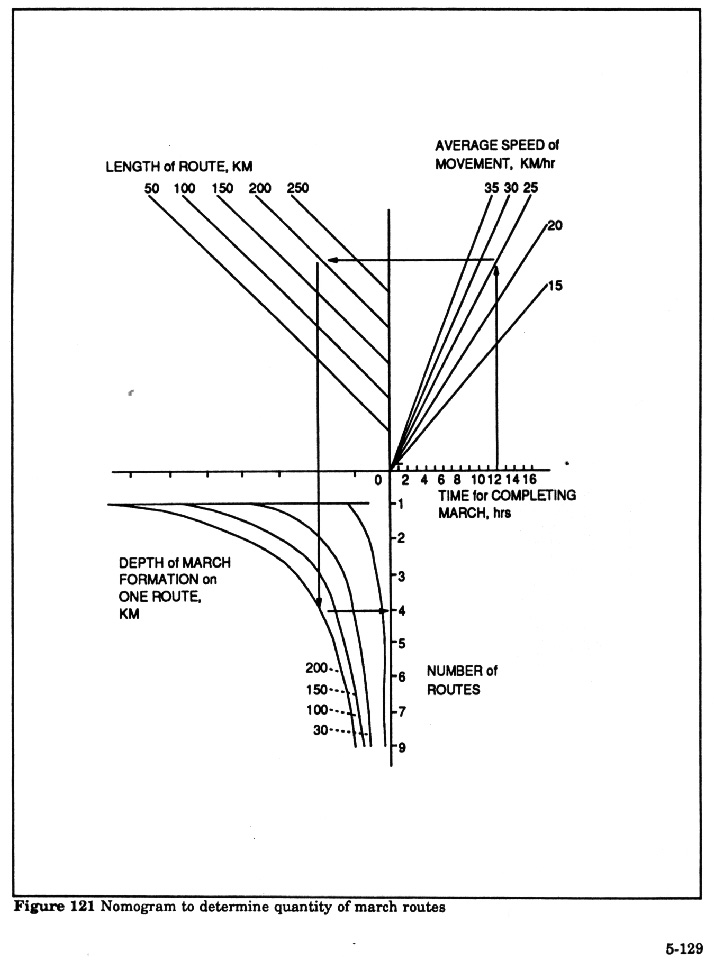
|
|
| |
Methods for Calculating Marches in
Complex Situations
March decision-making and planning, change in the order of march with an abrupt
situation change, as well as deployment of columns, all involve laborious
computations. On one hand it is necessary to compute different variants in
order to compare and select the optimal variant; on the other hand the selected
variant must be worked out in detail.
A march computation is performed usually in stages. First one determines the
approximate values of the basic march indices required by the commander for a
comparative analysis of various possible variants. The commander performs these
calculations personally or jointly with his chief of staff (staff officers).
The calculation variant selected by the commander can be adopted by his staff
officers as a basis for detailed elaboration (on the commander's map and their
working maps) prior to the final march decision. This portion of the
calculations will be the final stage of the computation. Obviously the faster
it is completed the sooner the commander will be able to reach a
thoroughly-substantiated march decision covering all elements.
The success of a march also depends on how quickly the requisite calculations
are performed and decisions made by the commander pertaining to continuation of
the march under conditions of abrupt situation changes or when it is necessary
to deploy for combat directly from the march columns. The principal problems
which must be solved in deployment of troops from march formation include
determination of the distance at which columns following one another could line
up with column heads abreast, and the time required for this -- depending on
speed, length of columns and column lead. (Shown in Figure 122).
Calculations for drawing abreast or deploying columns during a march, manual
determination of requisite distances, time, or speeds are performed according
to the following formulas.
For example, the distance (1) at which the head of column B will be abreast of
the head of column A can be computed with formulas: l=( V1 x S)
÷ (V2 - V1 ) (1)
or l=S ÷ (K - l) (2)
Where l=distance at which column B reaches the head of column A; V1
and V2 -- speeds of columns A and B (respectively); S=lead between
columns A and B (or vehicles A and B); K -- Coefficient indicating the ratio of
column speeds --V2 ÷ V1.
The time (t) it takes for the heads of columns A and B to stand abreast is
determined with formulas
t=l ÷ V1 (3) or t=l + S ÷V (4)
If the distance l was not determined (or does not need to be determined), and
it is necessary to determine only the time required for the columns to stand
abreast, it may be obtained with formula:
l=S ÷ (V1 (K - l)). (5)
Example problem: at what distance (l) and how much time will it take for the
head of column B to reach a point abreast of the head of column A if the first
column (A) proceeds at a speed of V1=16 km/h, while the second
column (B) can proceed at a speed of V2=24 km/h and if the lead (S)
between column B is 8 km (Fig 123).
|
|
| |
Figure 122 Conditions of
formation shift (a) and deployment (b) of columns on a march
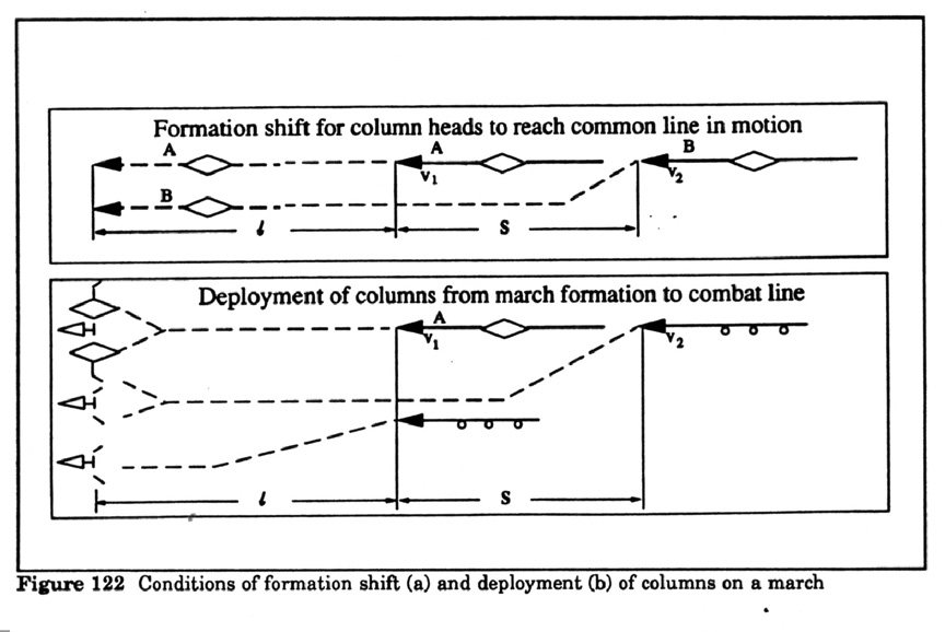 |
|
| |
Figure 123 Formation change of columns in
movement
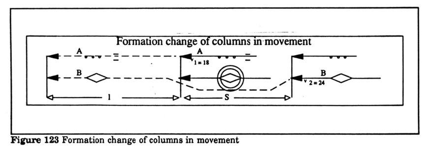
|
|
| |
Figure 124 Relationship between speed, time,
and distance rqeuired for columns to move from sequence head to tail into line
abreast
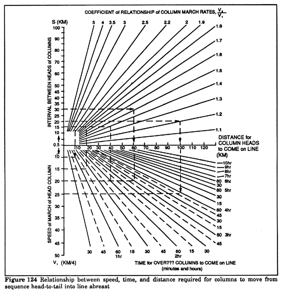
|
|
| |
Figure 125 Values of
coefficient K
|
Values of Coefficient K=V2 ÷ V11
|
|
17 |
20 |
22 |
25 |
27 |
30 |
32 |
35 |
37 |
40 |
42 |
45 |
47 |
50 |
60 |
| 10 |
1.7 |
2 |
2.2 |
2.5 |
2.7 |
3.0 |
3.2 |
3.5 |
3.7 |
4.0 |
4.2 |
4.5 |
4.7 |
5.0 |
6.0 |
| 12 |
1.4 |
1.7 |
1.8 |
2.1 |
2.2 |
2.5 |
2.7 |
2.8 |
3.0 |
3.3 |
3.5 |
3.7 |
3.9 |
4.2 |
5.0 |
| 15 |
1.1 |
1.3 |
1.5 |
1.7 |
1.8 |
2.0 |
2.1 |
2.3 |
2.5 |
2.7 |
2.8 |
3.0 |
3.1 |
3.3 |
4.0 |
| 17 |
1.0 |
1.2 |
1.3 |
1.5 |
1.6 |
1.8 |
1.9 |
2.0 |
2.2 |
2.3 |
2.5 |
2.6 |
2.8 |
3.0 |
3.5 |
| 20 |
- |
1.0 |
1.1 |
1.2 |
1.3 |
1.5 |
1.6 |
1.7 |
1.8 |
2.0 |
2.1 |
2.2 |
2.3 |
2.5 |
3.0 |
| 22 |
- |
- |
1.0 |
1.1 |
1.2 |
1.4 |
1.5 |
1.6 |
1.7 |
1.8 |
1.9 |
2.0 |
2.1 |
2.2 |
2.4 |
| 25 |
- |
- |
- |
1.0 |
1.1 |
1.2 |
1.3 |
1.4 |
1.5 |
1.6 |
1.7 |
1.8 |
1.9 |
2.0 |
2.4 |
| 27 |
- |
- |
- |
- |
1.0 |
1.1 |
1.2 |
1.3 |
1.4 |
1.5 |
1.6 |
1.7 |
1.8 |
1.9 |
2.2 |
| 30 |
- |
- |
- |
- |
- |
1.0 |
1.1 |
1.2 |
1.2 |
1.3 |
1.4 |
1.5 |
1.6 |
1.7 |
2.0 |
|
|
| |
Substituting specific data in formula (1):

|
|
| |
we find that:
l=(16 x 8) ÷ (21 - 16)=16 km
According to formula (3): t=l ÷ V1
we find that t=16 ÷ 16=1 hr
But in this example the question can also be stated differently. For example,
we must determine the speed (V2) at which column B must move in
order to reach a position abreast of column A in 1 (2, 3, etc) hour, or by
covering a distance of 16 (20, 30, etc) km. This problem is solved with the
above formulas by substituting known quantities.
These formulas can be used to solve any of the above problems fairly rapidly.
They can be solved even faster and more simply, however, by utilizing the
nomogram (Figure 3).
With the aid of the graph one can quickly find such quantities as 1 and t with
various values of S and column or vehicle speeds (V). The sequence of use is
shown in this example. Assume that we wish to determine at what distance,
1, and in what time, t, column B (following
behind column A) will reach a position abreast of column A if the column lead
(S) is 30km, the first column (A) is traveling at 20 km/h, and the second
column (B) is proceeding at 30 km/h.
First find index K, that is the ratio V2 ÷ V1. In
this case K=30:20=1.5. In order to speed up determination of index K with
various column speeds V1 and V2, use a table compiled in
advance.
Then find the values of 1 and t on the graph in Figure 3. For this, draw a
horizontal line from the mark "30 km" on line S to its point of
intersection with the diagonal line corresponding to index K=1.5, and from the
point of intersection draw a perpendicular line down to line 1. At the point of
intersection between the perpendicular line and line 1 find 1=60 km. This means
that column a will travel a distance of 60 km before column B reaches a
position abreast.
Time (t) is found on the same graph by drawing a perpendicular
line from point 1=60 km to the point of intersection with the horizontal line
designating speed V1 (in this case equal to 20 km/h). The point of
intersection of the perpendicular line and this line will show the time it will
take for column B to reach a position abreast of column a with the given ratio
and specific speeds; the time is found on diagonal line t at which the point of
intersection occurs. In our example t=3 hrs.
We can also use the graph top solve inverse problems such as determination of
the ratio of speeds V1 and V2 at which the columns can
reach a position abreast (or deploy for combat) in a give time or at a given
distance 1. For example, assume that we must determine at what ratio of speeds
(V1 and V2) two columns can be brought to a position
abreast if this must be accomplished in a distance 1=20 km, and the column lead
is S=10 km. In order to solve this problem draw a horizontal line from point
"10 km" on line S and a vertical line from point "20 km" on
line 1 to their point of intersection. Find in the region of this point of
intersection the closest diagonal line
K=V2 ÷ V1 .
In this example this point was on diagonal line K=1.5. This means that the two
columns can reach an abreast position with a ratio of column speeds of 1.5:1,
that is V2=5 V1.
We must stipulate that the graph can be utilized with sufficient accuracy in
all cases where the speed of the forward columns is at least 5 km/h, and the
column lead (S) is more than 5 km.
One typical problem which must be solved quickly is determination of time and
speeds for deployment of troops from march columns. In this case two indices
are taken for the basis of computation -- the distance (S) from the head of the
first column to the tail of the following column, if it is necessary for all
vehicles in these two (and more) columns to deploy, and the possible speed of
vehicles at the head and tail of these columns (that basis of road conditions
or distance 1 and available travel time (t). The graph enables one quickly to
determine all possible values of the sought quantities (1,V, and t) and to
determine the best variant on the basis of situation demands.
For example, determine the time (t) and speed (V1)
at which the lead vehicles of column A must travel if the vehicles at the tail
of column B can move at a speed (V2) not exceeding 30 km/h under
given road conditions; the length of each column is 8 km, and the column gap is
4 km (resulting in a total column length of S=20 km).
To solve this problem draw from the "20 km" point on the vertical
line of values s a horizontal line, intersecting all diagonal
lines indicating values of ratio
K=V2 ÷ V1.
From the points of intersection sequentially draw perpendicular lines to line 1
and continue them to the point of intersection with the horizontal lines of
various values of V1. At the points of intersection of the
perpendicular lines and lines 1 and V1 we find the specific values
of these quantities (1 and V1) for the corresponding ratio of K.
For example, for ratio K=3 (V2=30 km/h, V1=10 km/h) 1=10
km, t=1 hour; for ratio K=2 (V2=30 km/h, V1=15 km/h),
1=20 km, t=1 hour 20 minutes; for ratio K=1.5 (V2=30 km/h,
V1=20 km/h) 1=40 km, t=2 hours; for ratio K=1.2 (V2=30
km/h, V1=25 km/h) 1=100 km, t=4 hours. All these figures are
obtained on the graph within a few seconds, which makes it possible quickly t
asses different variants, selecting from them that which most corresponds to
the situation conditions.
Having determined the average speed, one must estimate capability to achieve it
in relation to the given conditions. One should proceed thereby from the
features of individual route sections, determining V average for each of these
sections. It may turn out that on some stretches speed is below the average
figure for a larger segment of the route, and possible for the entire march. In
this in the general form average speed is determined by formula V
average=Stot ÷ ttot.
 where Stot is the total length of the
route or individual (of significant length) route section, while
ttot is the time distance on that section, in calculating particular
values of V average one must proceed from road conditions:
This, differentiated approach to determining average speeds on route sections,
taking into consideration the required average value for the entire route, will
be the most correct. The fact is that in crossing obstacles all vehicles in the
column travel at the same speed; the lead vehicles (subunits) cannot increase
speed until the entire column has crossed the given obstacle. In order to
reduce the time required for this operation it is advisable to cross obstacles
with compressed columns, reducing the vehicle gap when approaching the obstacle
(1.7 km), while with a compressed column the obstacle can be crossed in almost
half the time. In march computations it is important to determine not how much
time will be required to cross a given obstacle but rather how much time will
be lost thereby. This approach simplifies calculations, since it is sufficient
to add the total time lost in crossing obstacles to the average travel time
index for the section (or for the entire route).
Footnotes
1. This discussion is taken from a recent Soviet article
"Modeling Battle" by Colonel P. Ulugbenikov
2. This very interesting calculation is the only major new
formula found in the new book Informatics in military affairs by A.
Vainer, published by DOSAAF in 1989. The publication of the book itself,
devoted to the use of computers and other methods for the practical application
of mathematical analysis by commanders to combat as a text for high school
students is an indication of the unrelenting Soviet effort to educate a new
generation in the scientific study of leading forces in combat.
3. Among recent discussions of this topic is the article
"Toward the question of the creation of strike groupings in offensive
operations" by General Major A. E. Tatarchenko in Military
Thought May, 1982. In addition to interesting theoretical issues the
article contains several useful formulas, one for determining the ratio of
widths of strike sector and total width of front in relation to the ratio of
correlation of forces in the strike sector and across the total front (see this
section here); the second for determining the relationship between initial and
final correlations and the losses of two sides; and this formula for the
relation of correlation of forces and advance rates.
4. This section is from an article "Method for
Evaluating Terrain Passibility", by Colonels V. Korneychuk, K. Lapshin,
and Ye. Galitskiy, which appeared in Voyennaya Mysl' in April 1967.
5. This section is taken from an article by Colonels
Korneychuk, Lapshin, and Galitskiy which appeared in Military Thought
in April 1967.
|
|